library(data.table); library(tidysynth)
m <- fread(here::here("materials/data/beanbuzz_markets.csv"))
m[, first_treat := ifelse(cohort_lab == "never", 0L, as.integer(cohort_lab))]
m[, log_rev := log(revenue)]
NG <- m[is_northgate == TRUE, unique(market_id)]   # "M17"
GO <- m[is_northgate == TRUE, unique(first_treat)] # 53
PRE <- 1:(GO - 1)

# (a) Northgate: build synthetic control (match lagged log_rev + market covariates)
# ___ YOUR CODE: so <- subdf |> synthetic_control(outcome=log_rev, unit=market_id, time=week,
#                       i_unit=NG, i_time=GO-1L, generate_placebos=TRUE) |>
#                       generate_predictor(...) |> generate_weights(optimization_window=PRE) |>
#                       generate_control()

# (b) read the post-period ATT off the gap, and the pre-RMSPE
# ___ YOUR CODE: ts <- so |> grab_synthetic_control(placebo=FALSE)  # real_y, synth_y by time
#                att <- mean(real_y - synth_y) over POST  -> +0.152

# (c) read the sparse unit weights
# ___ YOUR CODE: so |> grab_unit_weights()16 Session: Synthetic Controls
16.1 Lecture Slides
16.2 Overview
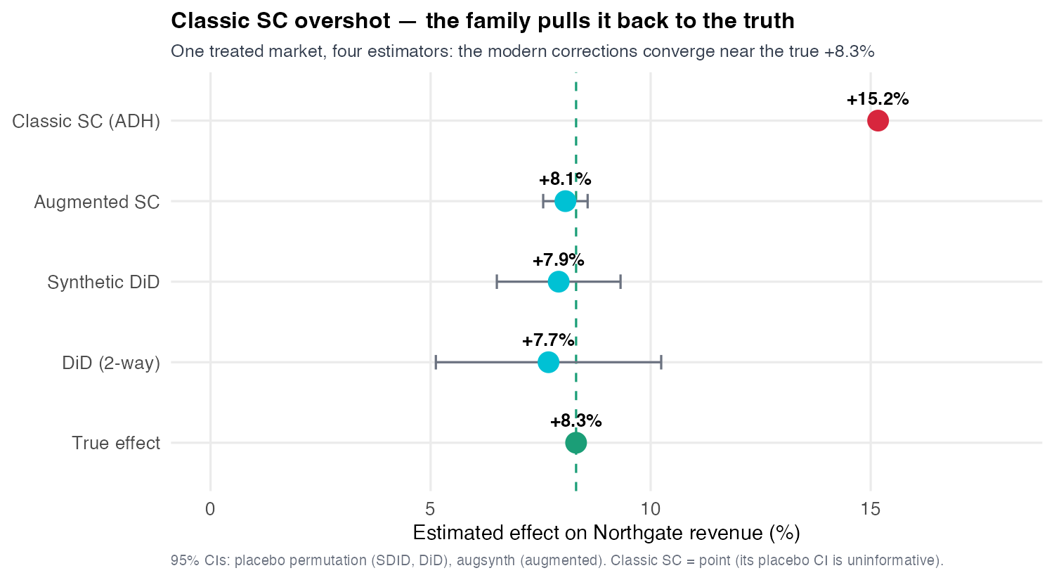
S10 answered “what is the app worth on average?”; BeanBuzz’s board now asks a sharper question — what did it do to Northgate, the flagship (market M17, the largest, seven stores, go-live week 53) — and that single-flagship question breaks the difference-in-differences machinery, because one treated unit has no cohort to average over and a lone pre-trend is mostly noise. Synthetic control answers it the Part V way — by imputing the missing \(Y(0)\), now as a convex blend of donor markets chosen to track Northgate before launch, the natural next step after S10 gave every clean control weight 1. The catch is that classic Abadie-Diamond-Hainmueller (ADH) synthetic control overshoots to +15.2% against a true Northgate effect of +8.3%. The reason is mechanical and exact: Northgate is the largest market, sitting at the edge of the donor convex hull, so no convex blend reaches its level. That leaves a +6.8% pre-period offset which leaks one-for-one into the post-period gap (+15.2% ≈ +6.8% offset + +8.3% true). The honest verdict that follows is deliberately non-triumphant: the placebo-in-space test ranks Northgate only 2 of 16 (Fisher \(p = 0.125\), one donor beats it) and the modern scpi prediction interval places the honest effect band at [+6.1%, +10.1%], so single-unit synthetic-control inference is fragile and must be corroborated. Corroboration comes from the modern family that pulls the overshoot back to the truth: augmented synthetic control closes the pre-fit offset and lands at +8.1% [+7.6%, +8.6%], synthetic DiD gives +7.9%, and plain DiD +7.7% — three methods with independent failure modes clustering on +8.3% while classic SC stands alone as the outlier. The unifying idea is that DiD, SC, and synthetic DiD are three corners of one weighted-DiD design (uniform-on-both, units-only, both axes), and the weight vectors that build each imputation are the rows of a low-rank matrix. Two through-lines tie the session to its neighbours: back to S10 (the identical honest-uncertainty discipline — a point estimate without a band is not a finding) and forward to S12 (weights become a matrix, and DiD / SC / SDID / unconfoundedness become one matrix-completion problem under different regularizers).
Learning objectives. By the end of this session you will be able to:
- Construct a synthetic control for a single treated unit — a convex donor blend (\(\omega\) in the simplex) — and read it as imputing the never-observed \(Y(0)\), explaining why the single-flagship case defeats cohort-based DiD.
- Diagnose a synthetic-control fit: show how an imperfect pre-fit inflates the estimate (Northgate +15.2% = +6.8% hull-driven offset + true +8.3%) and why, per Ferman, a perfect pre-fit is necessary but never sufficient.
- Infer honestly with placebo-in-space (rank 2/16, \(p = 0.125\)) and an scpi prediction interval ([+6.1%, +10.1%]) — reproducing the SC point to the digit in both R and Python (the graded bilingual step).
- Reconcile classic, augmented, synthetic-DiD and plain DiD in one estimator forest, locating the three corners of a single weighted-DiD design and pulling the +15.2% overshoot back to the true +8.3%.
- Read the unit and time weight vectors as the rows of a low-rank matrix, and see why stacking those rows hands S11 off to S12’s matrix-completion view (DiD / SC / SDID as one problem under different regularizers).
16.3 Lecture Notes
16.3.1 The single-flagship question breaks the DiD machinery
16.3.1.1 From a portfolio average to one unit
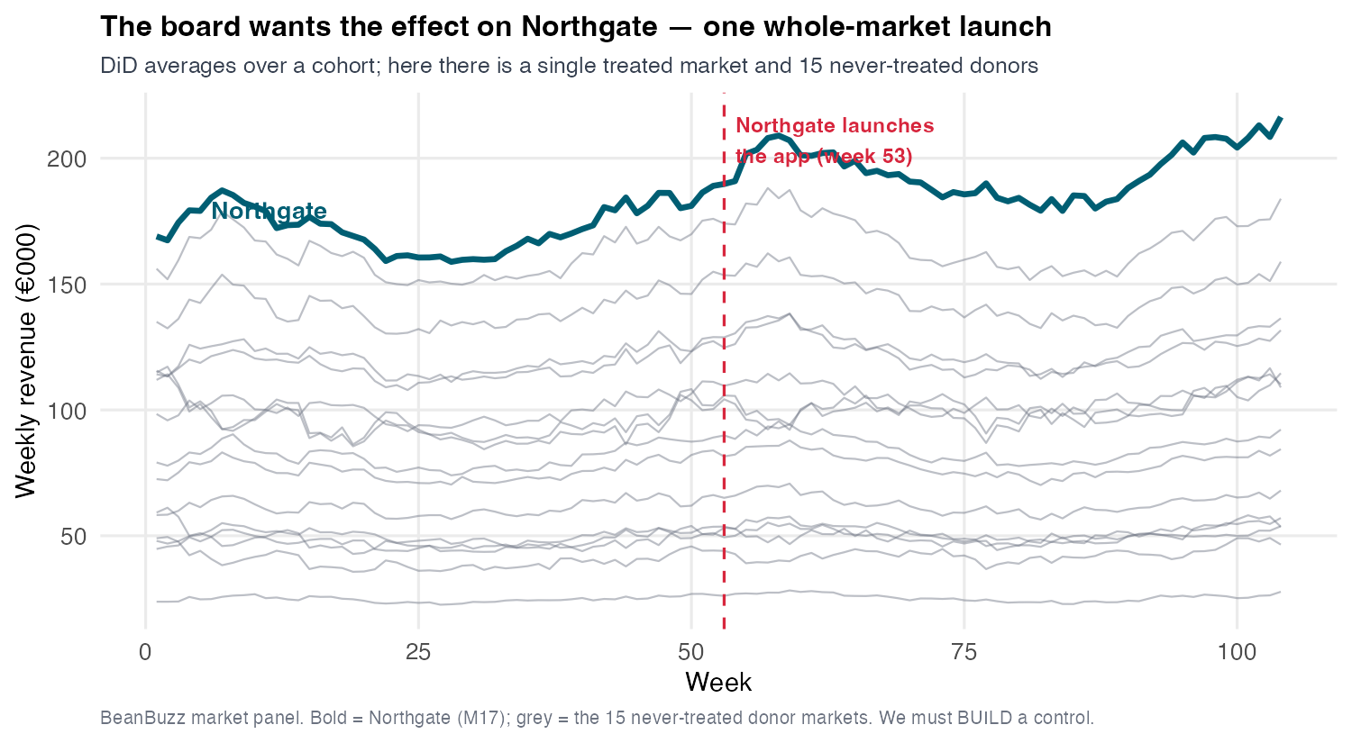
S10 delivered a portfolio answer — the overall ATT across all treated BeanBuzz markets, roughly +5%, close to the true overall effect of +4.9%. But a board does not run a portfolio; it runs flagship decisions. The question now is narrow and concrete: what did the loyalty app do to Northgate specifically — market M17, region 4, urban, the single largest market with seven stores, launched in the first wave at week 53 of 104 (Figure 16.1). The donor pool is fixed and clean: the 15 never-treated markets, observed across all 104 weeks. Notice already in the raw picture that Northgate (bold) sits above the donor fan even before launch — it is the biggest market, at the edge of the pack. That edge position is not a throwaway detail; it is the villain of Section 16.3.4, the reason a naive synthetic control will overshoot.
16.3.1.2 Why one treated unit has no purchase on parallel trends
Every robust DiD estimator in S10 leaned on cohorts — multiple units treated at similar times — so the group-time ATT averaged over many treated units and parallel trends was disciplined by a whole comparison pool. Northgate is one unit. A single unit’s pre-period trajectory is mostly idiosyncratic noise, so the question “are the treated and control trends parallel?” has almost nothing to constrain it: with one treated line, any donor average can be made to look parallel or not depending on which donors you pick. There is no cohort to average over, no way to borrow strength across treated units. To be precise, the number is not the problem — a plain 2×2 DiD on Northgate already gives +7.7% (true +8.3%). What fails at \(N = 1\) is defending it: no cohort, no clustered inference, no pre-test power. This is not a failure of DiD so much as a boundary — the boundary you hit the moment there is a single treated flagship. The constructive response is to stop asking every clean control to play the same role and instead build a tailored counterfactual: a weighted blend of donors chosen to track this unit.
16.3.1.3 The Part V spine, one more turn
Hold the spreadsheet image from S10 one more time: a panel of markets and weeks with a blanked-out rectangle for the never-observed \(Y(0)\) of the treated market after launch. Part V is one long project to impute that rectangle under a progressively weaker restriction on trends. S10 filled it with additive unit-plus-time effects (parallel trends); S11 fills it with a weighted blend of donor markets; S12 will fill it with a flexible factor model. The single sentence to carry through the session: difference-in-differences is the special case that gives every clean control the same weight, 1; synthetic control asks the next question — which donors, and how much weight on each. Synthetic control is the first method to actually solve for those weights — that is today’s work; synthetic DiD later in the session will solve for weights on both axes at once.
16.3.1.4 A weighted control is a synthetic unit
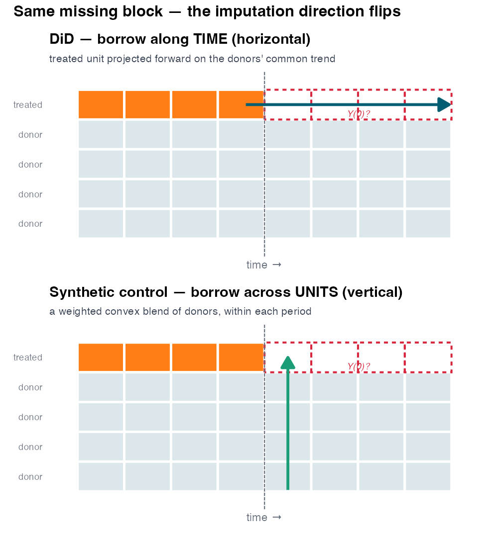
DiD and synthetic control are the same idea — impute \(Y(0)\) from controls — differing only in the weights, and that one change flips the direction of the imputation. DiD borrows horizontally — it projects the treated unit forward in time on the donors’ common trend. Synthetic control borrows vertically — each missing post-period cell is a weighted column of donors (Figure 16.2). DiD implicitly assigns every clean control the same weight (a simple average) and asks the treated unit to have moved in parallel with that average. Synthetic control instead solves for the weights: it searches over convex combinations of donors — weights that are non-negative and sum to one — to find the particular blend whose pre-treatment trajectory most closely matches the treated unit’s. That weighted blend is a synthetic Northgate: a fictional market assembled from real donors, standing in for the one we cannot observe after launch. After treatment, when the real Northgate’s \(Y(0)\) is unobservable, the synthetic unit keeps tracking forward and serves as the counterfactual. The convexity restriction (Section 16.3.2) is the method’s signature design choice — and, for Northgate, its central limitation.
16.3.2 The ADH construction: choose weights in the simplex
16.3.2.1 The objective and the simplex
Abadie-Diamond-Hainmueller’s move is to choose donor weights \(\omega\) that make the synthetic unit’s pre-treatment outcome path track the treated unit’s — match the trajectory, the thing we actually want to extrapolate, not just a list of covariate means (Abadie, Diamond, and Hainmueller 2010). With \(T_0\) pre-treatment periods, donors indexed by \(j\), and outcomes \(Y\):
\[\min_{\omega}\ \sum_{t \le T_0}\Big(Y^{\text{treat}}_t - \sum_{j}\omega_j\,Y^{\text{donor}}_{j,t}\Big)^2 \quad \text{s.t. } \omega_j \ge 0,\ \textstyle\sum_j \omega_j = 1. \tag{16.1}\]
The two constraints — non-negative weights that sum to one — make \(\omega\) a point in the simplex, and the synthetic unit a convex combination of donors. Covariates and lagged outcomes can be folded into the matching as additional predictors (the labs match on market size, urban share, store count, and four lagged log-revenue snapshots), but the pre-period outcome path is the dominant target; keep the focus there.
16.3.2.2 Convexity = no extrapolation, with a cost
This convexity is the method’s virtue and its curse (Abadie 2021). Its virtue: forbidding negative weights and weights above one means the synthetic unit is an interpolation of observed donors — it never extrapolates beyond the range of behaviour any donor actually exhibited, which guards against the wild out-of-sample predictions unconstrained regression can produce. Its cost, which Section 16.3.4 will hit hard: if the treated unit lies outside the convex hull of the donors — for instance, if it is the largest market and no blend of smaller donors can match its level — then no convex weighting can fit it, and the residual pre-period misfit becomes bias. This is not a tuning problem you can fix by trying harder inside the simplex; it is the simplex itself.
16.3.3 The Proposition-99 warm-up: what a clean fit looks like
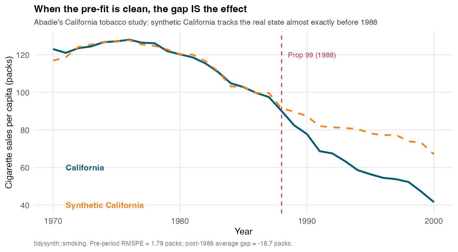
Ground the method in the case that made it famous, because it shows what a good fit looks like before we meet a bad one. Abadie, Diamond and Hainmueller studied California’s Proposition 99, the 1988 tobacco tax, asking what happened to per-capita cigarette consumption (Abadie, Diamond, and Hainmueller 2010, 2015). They built a synthetic California from a convex blend of other US states chosen to match California’s pre-1988 smoking trajectory and predictors. The fit is the textbook ideal (Figure 16.3): before 1988 the synthetic line lies almost exactly on top of real California, with a pre-treatment root-mean-squared prediction error (pre-RMSPE) of roughly 1.8 packs per capita — small relative to the scale. Why does it fit so well? California, though large, sits comfortably inside the convex hull of the other states on the smoking dimension, so a blend can match it. Contrast this deliberately with Northgate, which does not sit inside its donors’ hull.
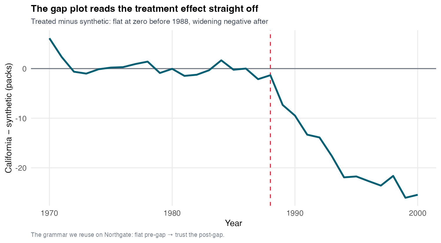
The standard synthetic-control read is the gap plot: subtract synthetic from real and plot the difference over time (Figure 16.4). Before treatment, a good fit means the gap hovers at zero — that flatness is the visual proof the synthetic unit is a faithful stand-in. After treatment, the gap is the estimated treatment effect at each period: for Prop 99 it opens steadily downward to about −18.7 cigarettes per capita by the late 1990s, a large and growing reduction. The crucial inferential point, which Section 16.3.4 exploits: the gap plot is only interpretable if the pre-period gap is flat at zero. A flat pre-gap licenses reading the post-gap as the effect; a non-flat pre-gap means the synthetic unit never matched the treated unit in the first place, so the post-gap mixes the true effect with the pre-existing misfit.
16.3.4 Northgate overshoots: an imperfect pre-fit leaks straight in
16.3.4.1 The diagnostic fit
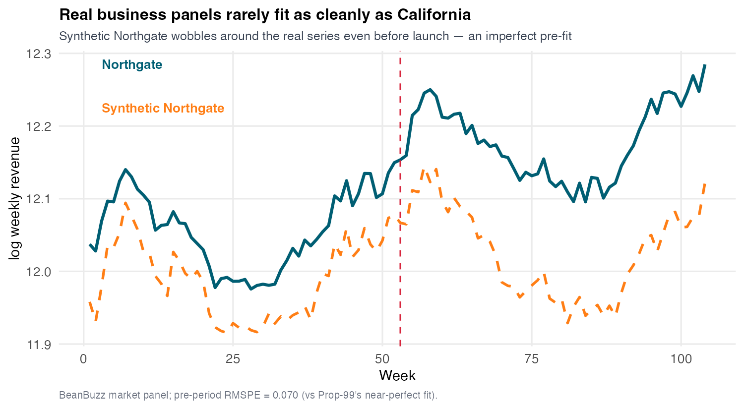
Run the identical ADH recipe on Northgate — donor pool the fifteen never-treated markets — and the pre-period fit is visibly worse than California’s (Figure 16.5): the synthetic line sits persistently below real Northgate even before week 53, never quite reaching its level. The reason is the convexity constraint colliding with Northgate’s position. Northgate is the largest market in the portfolio; every donor is smaller. A convex blend — weights summing to one, none negative — can only produce a synthetic unit whose level lies between the donors’ levels, so it cannot reach above all of them. Northgate sits at the edge of (effectively outside) the convex hull, and no convex weighting can match a point outside the hull. The result is a structural pre-period offset: the synthetic is biased low throughout.
16.3.4.2 The exact decomposition
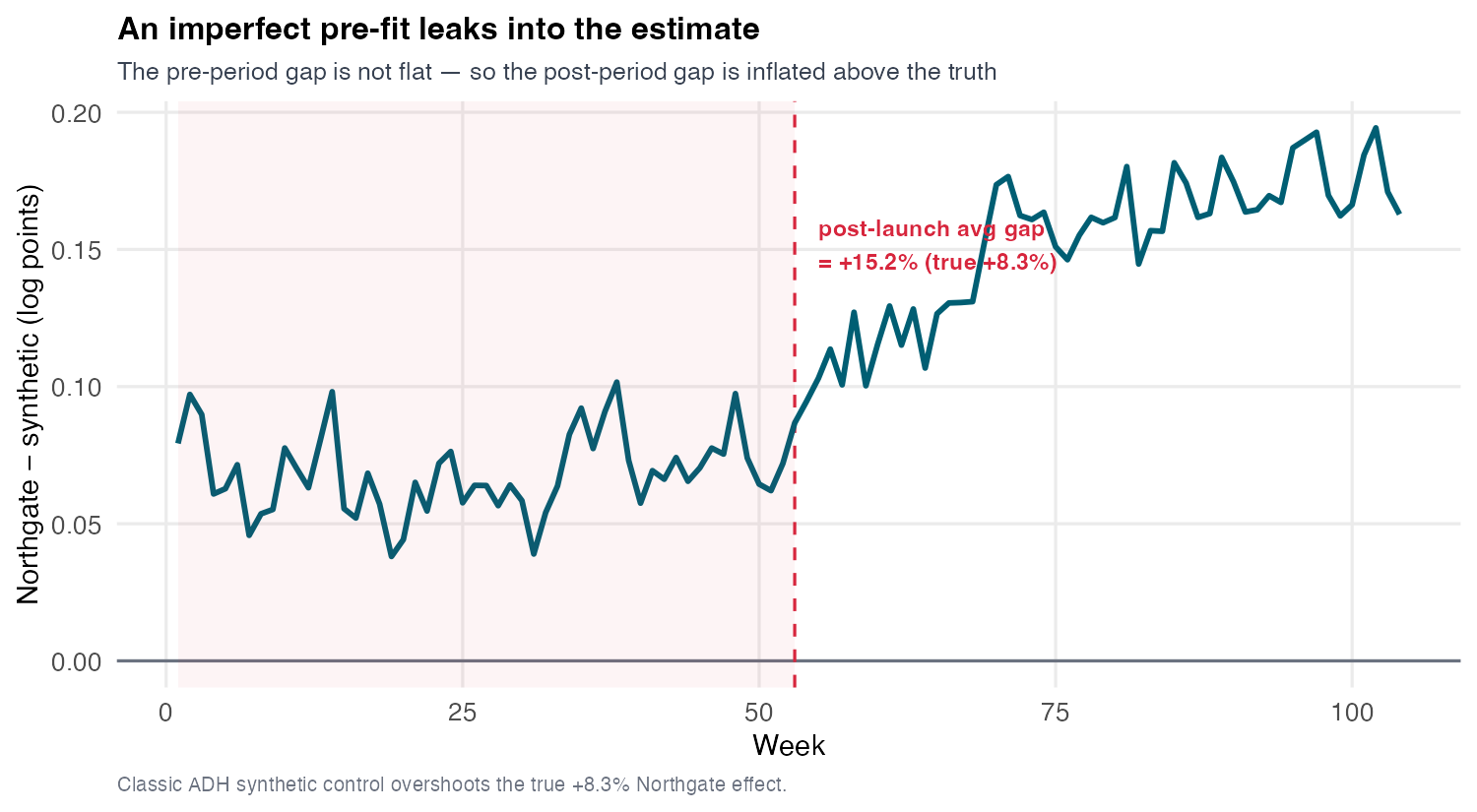
This is the mechanical heart of the session — the single most important arithmetic. Because the synthetic Northgate sits about 6.8% below the real one throughout the pre-period (pre-RMSPE ≈ 0.070), the gap plot does not start at zero — it starts at +6.8% (Figure 16.6). That baked-in offset does not vanish at launch; it persists into the post-period and adds to whatever true effect there is. So the post-period gap of +15.2% decomposes almost exactly into the pre-period offset plus the true Northgate effect:
\[\underbrace{+15.2\%}_{\text{classic SC post-gap}} \;\approx\; \underbrace{+6.8\%}_{\text{pre-period offset (edge of hull)}} \;+\; \underbrace{+8.3\%}_{\text{true Northgate effect}}. \tag{16.2}\]
Say this slowly: the classic SC overshoots not because the effect is large but because the fit is bad, and a bad fit contaminates the estimate one-for-one. This is the synthetic-control analog of S10’s contamination story (there a too-low estimate dragged down by forbidden comparisons; here a too-high estimate inflated by a pre-period offset), and it reframes the gap plot’s pre-period as a diagnostic you must check before trusting any number. Everything in Section 16.3.7 is about killing that +6.8% offset.
16.3.4.3 The weights collapse onto one donor — and a seed for S12
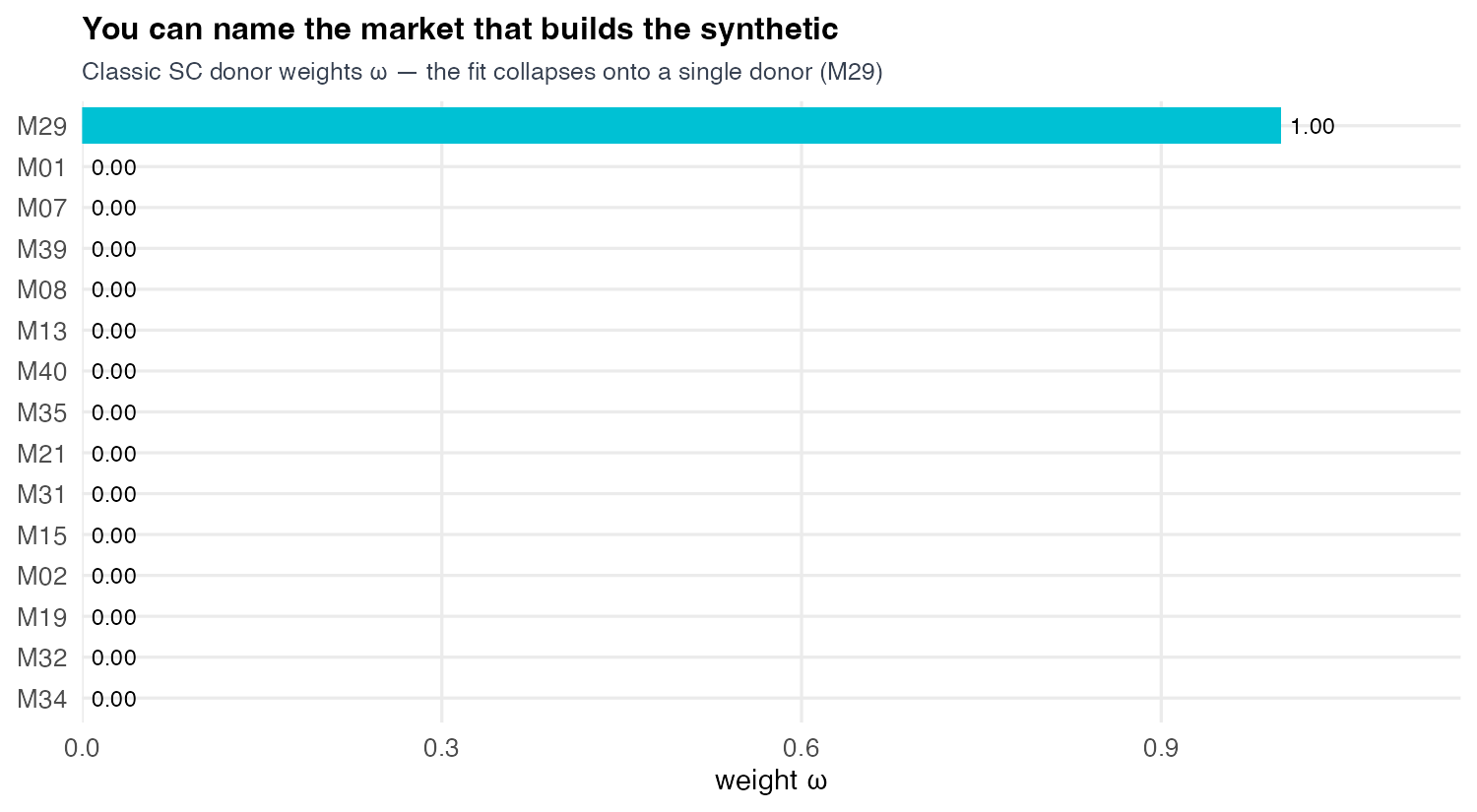
Read the blend (Figure 16.7). Synthetic-control weights are typically sparse — the simplex constraint plus the optimization load most of the weight onto a few donors and leave the rest at zero. Northgate’s classic fit is the extreme case: it is maximally sparse, collapsing almost entirely onto a single donor, market M29 (weight approx 0.9998), with every other market at zero. Sparsity is still the interpretability that makes synthetic control attractive to a board — you can name the one market your synthetic Northgate is made of and sanity-check it (does M29 share Northgate’s region, urbanicity, size?). Plant the S12 seed quietly: even this single-donor vector is one row of instructions — how to reconstruct one unit’s outcome path from the others. In Section 16.3.10 we stack such rows and recognize them as a low-rank matrix.
16.3.5 Placebo-in-space inference, and honest fragility
16.3.5.1 One treated unit has no standard error
The post-gap is +15.2% — but is it distinguishable from noise? Classical inference cannot say. A standard error needs repeated sampling or many treated units to average over; synthetic control on Northgate has neither — a single treated market, a single realized path, no replication. Abadie’s answer is not a standard error but a randomization (Fisher permutation) test (Abadie, Diamond, and Hainmueller 2010): if the treatment had no effect, the treated unit’s post-period gap should look like a typical donor’s gap when you pretend that donor was treated. The placebo-in-space recipe has three steps:
- Reassign treatment to each donor in turn, as if it launched at week 53.
- Score each unit by its MSPE ratio — post-period mean-squared gap divided by pre-period mean-squared gap — after re-running synthetic control for that placebo donor on the remaining pool.
- Rank every unit by that ratio; Northgate’s rank divided by the number of units is the Fisher \(p\)-value.
MSPE is the mean squared gap between a unit and its synthetic over a window. Dividing post by pre asks whether the gap grew after treatment relative to the pre-fit — so a placebo whose synthetic never tracked it (large pre-MSPE) cannot top the ranking just by being noisy, and a unit with a tight pre-fit but a modest post-gap can rank high. A common refinement (the fit-filter the lab reports) drops placebos whose pre-period MSPE exceeds 5x the treated unit’s before ranking.
16.3.5.2 The honest verdict
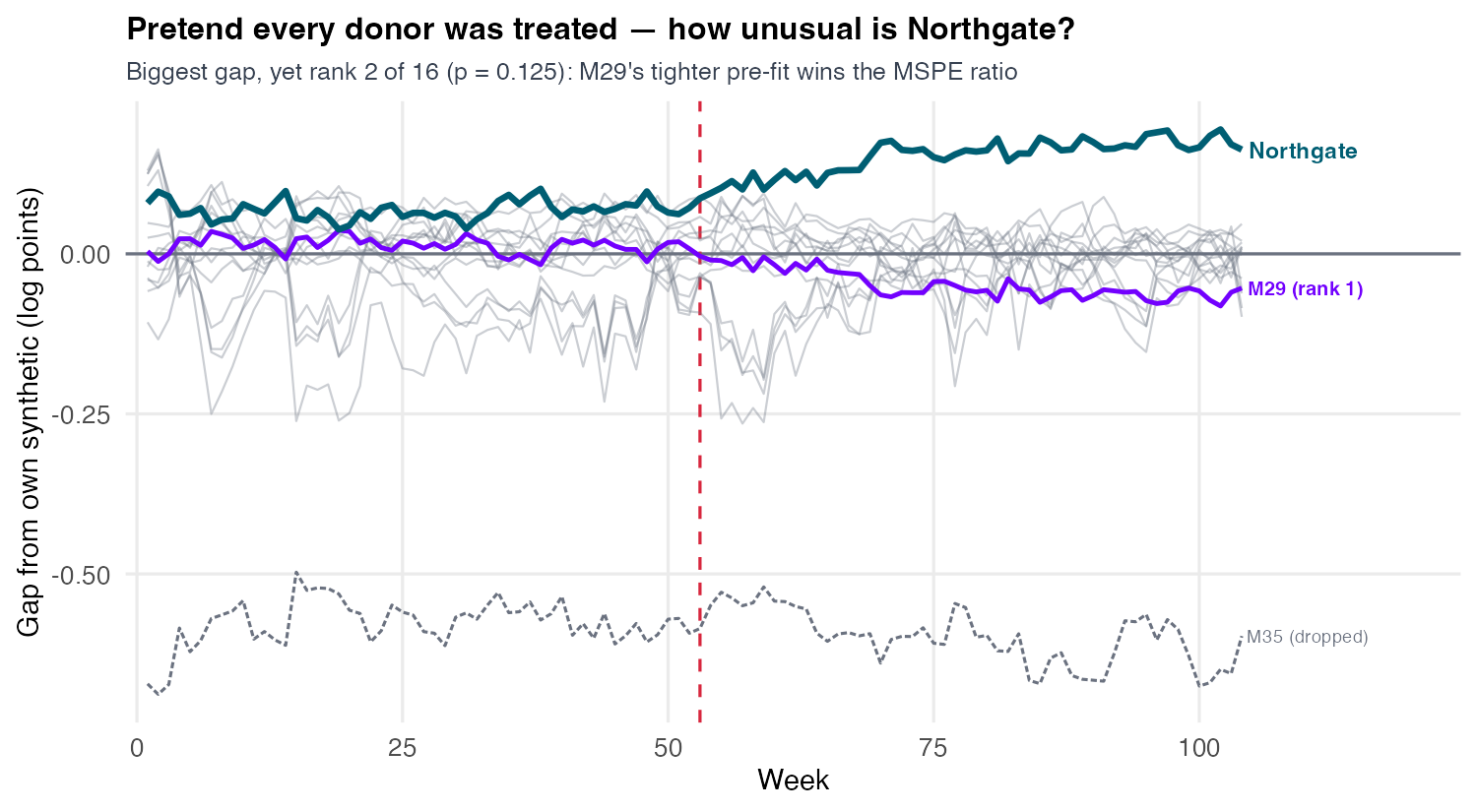
Northgate’s post-launch gap is the largest in the fan and visibly opens upward (Figure 16.8), but in the placebo fan it ranks only 2 of 16 — because the ranking statistic is the MSPE ratio, not the raw gap; Northgate’s post-launch gap is actually the largest in the fan. Donor M29 has a tiny post-gap but a near-perfect pre-fit (pre-MSPE approx 0.0003), so its ratio (approx 8.3) exceeds Northgate’s, whose imperfect pre-fit — the +6.8% hull-edge offset — deflates its ratio to approx 4.9. M29 outranks Northgate not because its effect is bigger but because the ratio rewards a tight pre-fit. The Fisher \(p\)-value is therefore 0.125 (rank 2 of 16); filtering out badly-fit placebos — like M35, whose pre-MSPE is approx 68x Northgate’s and is dropped by Abadie’s 5x fit-filter — leaves rank 2 of 15, \(p = 0.133\). By the conventional 0.05 bar, neither clears significance.
16.3.6 Modern prediction intervals: scpi and the honest band
The placebo test answers a ranking question — is the treated gap extreme among placebos — but it does not directly quantify how uncertain the counterfactual prediction is. Cattaneo, Feng, Palomba and Titiunik’s scpi framework does (Cattaneo et al. 2025): it constructs a genuine prediction interval around the synthetic unit’s predicted \(Y(0)\), decomposing the uncertainty into two pieces — the error in estimating the donor weights (in-sample) and the irreducible out-of-sample noise of predicting a future path. Formally, the synthetic counterfactual is \(\widehat{Y}^{(0)}_t=\sum_j \widehat{\omega}_j\,Y_{jt}\), and scpi reports a \((1-\alpha)\) prediction interval for that \(Y(0)_t\). The per-period effect is read as \(\widehat{\tau}_t = Y^{\text{obs}}_t - \widehat{Y}^{(0)}_t\), so the actual path lying above the whole band means \(\tau_t>0\). Stress the interpretation, because students will misread it: this is a band for the counterfactual \(Y(0)\), not a frequentist standard error attached to the point estimate. You read it by asking where the actual Northgate path falls relative to the band for its synthetic counterfactual.
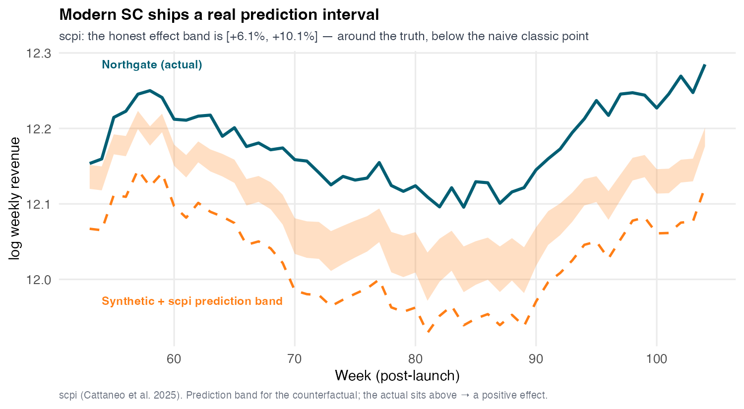
Read two things off the figure (Figure 16.9). First, the actual Northgate path sits above the prediction band for its counterfactual, which means there is a positive effect — the band does not contain “no effect” in a way that erases the result. Second, and this is the lesson, the honest effect band — actual minus the counterfactual prediction interval — is [+6.1%, +10.1%], centred near the true +8.3% and lying well below the naive +15.2% point. The naive point was overconfident, exactly because it inherited the +6.8% pre-offset (Equation 16.2). So scpi both confirms a positive effect and corrects the magnitude downward toward the truth: the interval reveals what the point hid. A conformal-inference alternative (Chernozhukov, Wüthrich, Zhu) gives a similar prediction guarantee under a permutation-style assumption — a different route, the same spirit (Chernozhukov, Wüthrich, and Zhu 2021).
16.3.7 Augmented SC: ridge bias-correction outside the hull
16.3.7.1 Relax the simplex, just enough
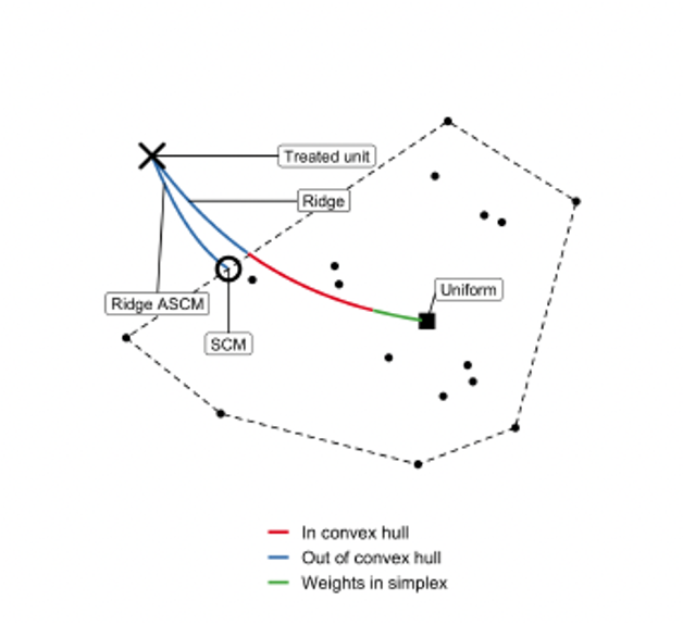
The +6.8% offset is a direct consequence of the simplex constraint: Northgate lies outside the donor convex hull, so no non-negative-weights-summing-to-one blend can reach it. Augmented synthetic control relaxes that constraint in a controlled way (Ben-Michael, Feller, and Rothstein 2021). It starts from the classic SC weights, then adds a ridge-regularized outcome-model correction for the remaining pre-treatment imbalance — in effect allowing the weights to step slightly outside the simplex (small negative or above-one weights) just enough to eliminate the residual misfit, with the ridge penalty preventing wild extrapolation. The cleanest analogy, which calls back to the matching session, is bias-corrected matching: match as well as you can, then run a regression to remove the leftover imbalance. Augmented SC does the same for trajectories.
16.3.7.2 Outcome model plus residuals: the doubly-robust form
Write the correction down. The augmented counterfactual is the classic SC prediction plus an imbalance-correction term, which rearranges into an equivalent doubly-robust form:
\[\widehat{Y}^{(0),\text{aug}}_{1T}=\underbrace{\sum_i \widehat{\omega}^{sc}_i\,Y_{iT}}_{\text{classic SC}}+\underbrace{\Big(\widehat{m}(X_1)-\sum_i \widehat{\omega}^{sc}_i\,\widehat{m}(X_i)\Big)}_{\text{imbalance correction}}=\underbrace{\widehat{m}(X_1)}_{\text{outcome model}}+\underbrace{\sum_i \widehat{\omega}^{sc}_i\big(Y_{iT}-\widehat{m}(X_i)\big)}_{\text{SC-reweighted residuals}} \tag{16.3}\]
The second line is AIPW-like, and that structure is exactly why augmented SC is doubly robust: if the SC weights already balance the pre-period the residual term vanishes in expectation, and if instead the outcome model \(\widehat{m}\) is correct the first term carries the estimate — you only need one of the two to be right. Here \(\widehat{m}\) is a ridge regression of the donors post-treatment outcomes on their centred pre-treatment outcomes, \(\widehat{m}(X)=\widehat{\eta}_0+X'\widehat{\eta}_x\), with penalty \(\lambda\) chosen by cross-validation over pre-periods. The ridge is what lets the effective donor weights leave the simplex (go slightly negative or above one) to reach a treated unit outside the hull (Figure 16.10), while the penalty stops the extrapolation running wild.
16.3.7.3 It works almost perfectly
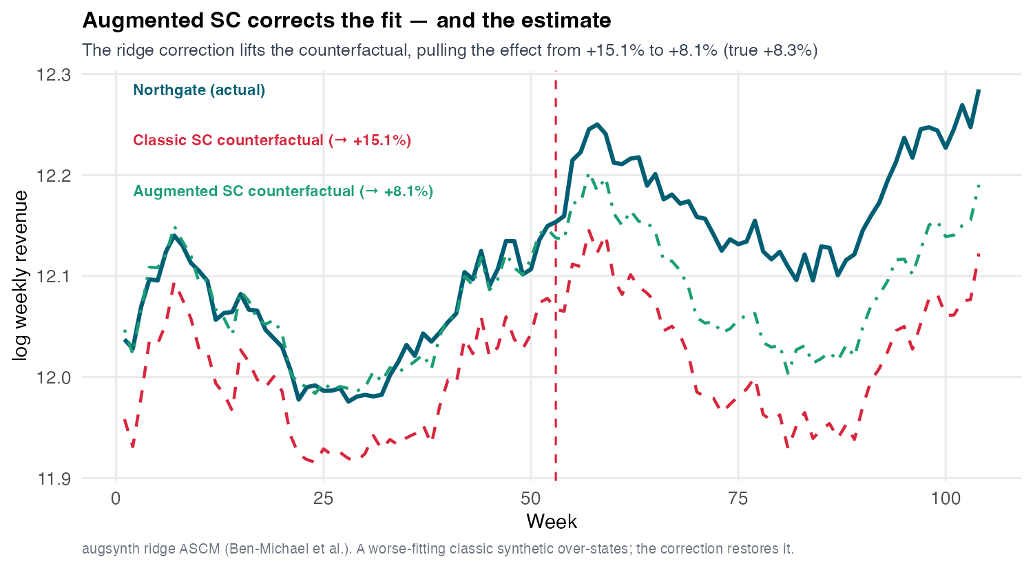
Closing the pre-fit collapses the overshoot (Figure 16.11). The augmented counterfactual lies essentially on top of real Northgate before week 53 — a near-perfect pre-fit, offset \(\approx 0.000\) — so the contamination term in Equation 16.2 vanishes and the estimate snaps back to +8.1% with a 95% confidence interval of [+7.6%, +8.6%], statistically indistinguishable from the true +8.3%. Walk the arc out loud: classic SC +15.2% (inflated by a bad fit) becomes augmented SC +8.1% (a good fit, the truth). This is the mirror of S10’s correction story — there a too-low estimate was pulled up toward the truth; here a too-high estimate is pulled down.
16.3.8 A good fit is not a free pass
16.3.8.1 The Ferman caution
Augmented SC just produced a near-perfect pre-fit and the right answer, which is seductive — it tempts you to treat pre-fit quality as proof of validity. Ferman’s caution says no (Ferman and Pinto 2021). When the donor pool is large relative to the length of the pre-period, the optimizer has enough free weights to drive the pre-period discrepancy to zero by fitting noise rather than capturing the structural relationship between treated and donor units — classic overfitting. Such weights fit the pre-period beautifully but project poorly into the post-period, so the counterfactual can be biased despite a flawless-looking fit. This is exactly parallel to S10’s “a flat pre-trend does not prove parallel trends”: there a flat pre-trend was evidence, not proof; here a flat pre-gap is evidence, not proof. Fit is a necessary condition for credibility, never a sufficient one.
16.3.8.2 Report three things, never one
The discipline that falls out is portable and identical to S10’s. Never report a synthetic-control point estimate alone — report three things:
- The fit — pre-period RMSPE and the gap plot (necessary, not sufficient; a bad fit like classic Northgate’s guarantees contamination).
- An interval — the scpi prediction band (Section 16.3.6) or the placebo \(p\)-value (Section 16.3.5) — quantifying how uncertain the counterfactual is.
- Cross-method agreement — do augmented SC, synthetic DiD, and plain DiD concur (read off the forest with placebo intervals, Figure 16.15, Section 16.3.9)?
Convergence across methods with independent failure modes is the real credibility check, exactly as it was in S10’s robust-estimator forest. This cashes the promise S10 made when it ended by telling students to “corroborate with synthetic control”: we have now built that corroboration, and the honesty rule transfers verbatim — a point estimate without a band and a robustness check is not a finding. Augmented SC’s bias-correction buys you the right point estimate, but it is not a substitute for the three-part report — the fit, the interval, and cross-method agreement together are the finding.
16.3.9 The bridge: units, time, or both
16.3.9.1 Three corners of one design
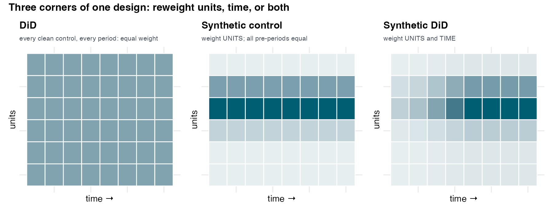
Look at the panel as a matrix of units by time. DiD and synthetic control each impute the missing \(Y(0)\) by weighting, but on different axes. DiD weights time: it implicitly treats every clean control unit equally (weight 1) and does its work through the period fixed effects, which capture the common time trend. Synthetic control weights units: it solves for bespoke donor weights \(\omega\) but treats every pre-period symmetrically. Each method fixes one axis (uniform) and optimizes the other — which makes the next step almost forced: if weighting units helps (SC) and weighting time helps (DiD’s period effects), why not do both? Arkhangelsky et al.’s synthetic difference-in-differences does exactly that (Arkhangelsky et al. 2021): solve for unit weights \(\omega\) and time weights \(\lambda\), then run a weighted two-way DiD. Writing the three estimators as one weighted two-way fixed-effects fit makes the family explicit — they differ only in the weights \((\omega, \lambda)\) they place on units and periods:
\[ \begin{aligned} \textbf{DiD:} &\quad \omega_j = \tfrac{1}{N_{\text{co}}},\ \lambda_t = \tfrac{1}{T_0} \quad &&\text{(uniform on both axes)}\\ \textbf{SC:} &\quad \omega_j \in \text{simplex},\ \lambda_t = \tfrac{1}{T_0} \quad &&\text{(sparse on units, uniform on time)}\\ \textbf{SDID:} &\quad \omega_j \in \text{simplex},\ \lambda_t \ \text{solved} \quad &&\text{(sparse on both axes)} \end{aligned} \tag{16.4}\]
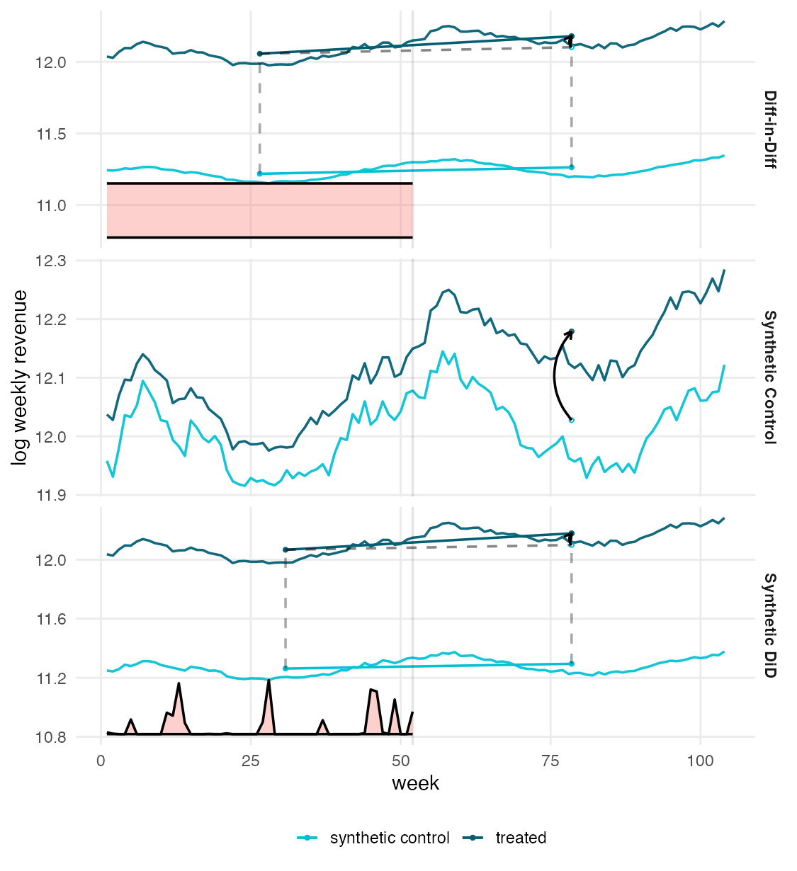
The two SDID weightings buy robustness to the two failure modes we have seen (Figure 16.12). The unit weights \(\omega\) make donors resemble the treated unit, relaxing the parallel-trends requirement — you no longer need the raw donor average to move in parallel, only the matched blend. The time weights \(\lambda\) up-weight the pre-periods that most resemble the post-period, relaxing the perfect-pre-fit requirement — small residual misfit on irrelevant pre-periods is down-weighted rather than leaking into the estimate. The headline property is SDID’s double robustness: it needs neither a perfect SC pre-fit (which Northgate cannot achieve in the simplex) nor exact parallel trends (which the omitted regional-economy factor violates) — get either the unit weights or the time weights right and the estimate holds, the same insurance logic as augmented SC’s AIPW correction (Equation 16.3).
16.3.9.2 DiD, SC, and SDID are one weighted regression
Write the family as a single weighted two-way fixed-effects regression. Synthetic DiD solves
\[(\widehat\tau^{\,sdid},\widehat\mu,\widehat\alpha,\widehat\beta)=\arg\min_{\tau,\mu,\alpha,\beta}\ \sum_{i}\sum_{t}\big(Y_{it}-\mu-\alpha_i-\beta_t-D_{it}\,\tau\big)^2\,\widehat\omega_i\,\widehat\lambda_t \tag{16.5}\]
where \(\mu\) is the intercept, \(\alpha_i\) the market (unit) effects, \(\beta_t\) the week (period) effects, \(D_{it}=1\) for the treated market post-launch, and \(\tau\) the ATT. The three estimators are this one regression (Equation 16.5) under different settings:
| Estimator | Unit FE \(\alpha_i\) | Unit weights \(\omega\) | Time weights \(\lambda\) |
|---|---|---|---|
| DiD | yes | uniform | uniform (both drop out) → plain TWFE |
| SC | omitted | in simplex | uniform |
| SDID | yes | in simplex | solved |
All three keep the period effects \(\beta_t\) — DiD’s time leverage, the common trend, present in every column and not a time weight. They differ only in whether the unit fixed effect \(\alpha_i\) is kept and which of \(\omega,\lambda\) are non-uniform.
16.3.9.3 SDID lands near the truth
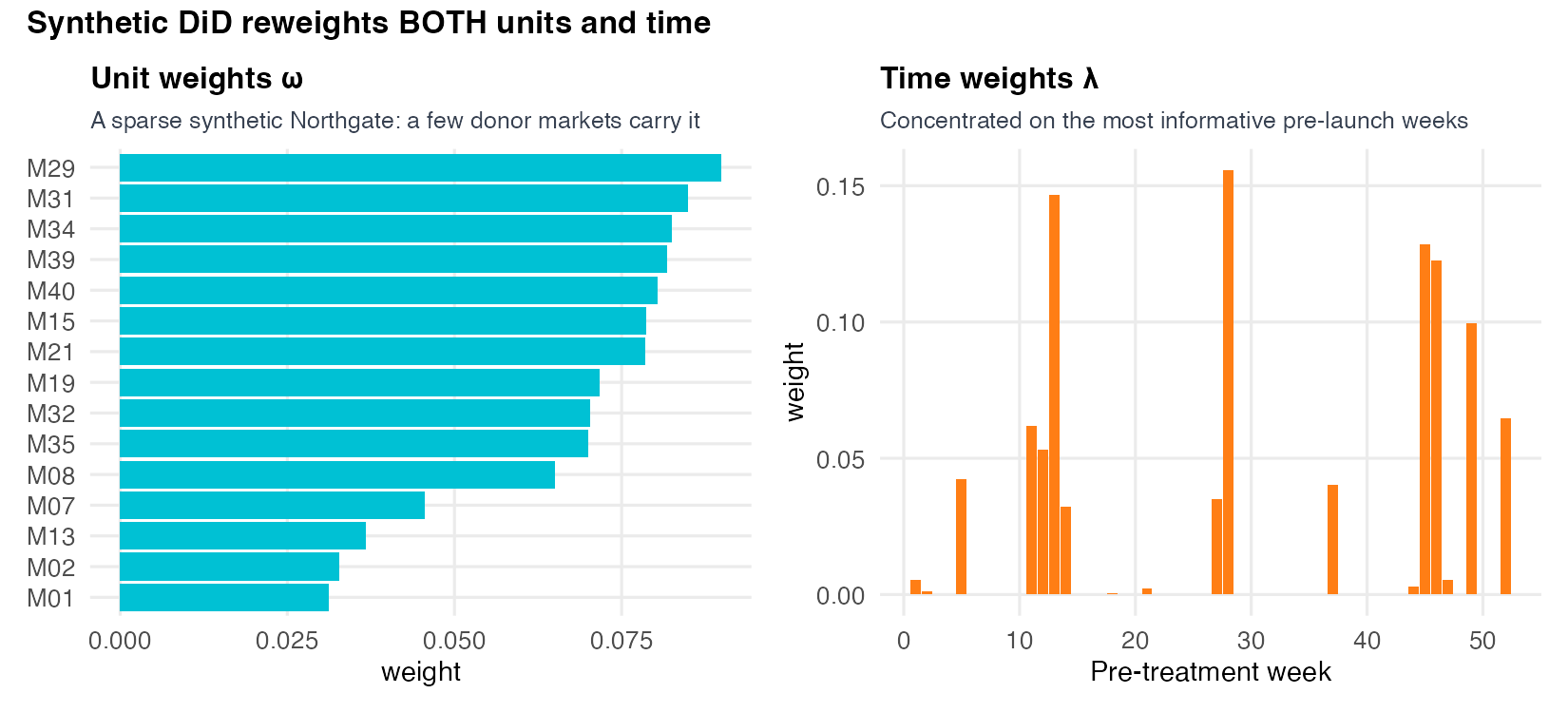
The two weight vectors in Figure 16.13 — now we know what they buy — give synthetic DiD +7.9% on Northgate against the true +8.3%; even plain DiD on Northgate gives +7.7%, also near the truth. The striking contrast: classic SC, insisting on a perfect convex fit it cannot achieve, overshoots to +15.2%, whereas SDID, which does not require a perfect fit, lands at +7.9%. The robustness of SDID comes precisely from not betting everything on one axis.
16.3.9.4 Watch SDID stay parallel where classic SC drifts
Placed in a forest (Figure 16.15), the verdict that the single \(p\)-value could not deliver appears as convergence: against the true +8.3%, augmented SC (+8.1% [+7.6, +8.6]), synthetic DiD (+7.9% [+6.5, +9.3]) and plain DiD (+7.7% [+5.2, +10.2]) each carry a 95% interval that contains the truth and cluster tightly, while classic SC sits alone at +15.2% as a bare point (no interval — inflated by the +6.8% pre-offset) — exposed as the one that trusted a bad fit. Reconcile the two sessions explicitly: S10’s portfolio-wide robust ATT was +4.9% (the average market); Northgate, the flagship, has a larger effect (+8.3%), and the family of estimators recovers it. The classic SC’s +15.2% was the Northgate analog of S10’s naive +16.3% — a headline number demolished by discipline.
16.3.10 From weights to a low-rank matrix: the S12 on-ramp
16.3.10.1 The weight vectors are a matrix in disguise
Two families, one ledger — the connective tissue of Part V, reused in S12 and the A5 memo:
| Family | What it buys | What it costs |
|---|---|---|
| Parallel-trends (S10 — DiD, CS, BJS) | Additive, transparent, cheap; borrows strength across a whole cohort. | Blind to a unit-specific, time-varying factor; needs a credible cohort and testable pre-trends. |
| Hull + loadings (S11 — SC, augmented SC, SDID) | Relaxes parallel trends; a unit-specific counterfactual that works at \(N=1\). | Needs the treated unit inside the donor hull and a non-overfit pre-fit; single-unit inference is weak. |
Go back to the “weights are a row” seed from Section 16.3.4. Every imputed \(Y(0)\) cell is a weighted combination of other cells in the panel — that is literally what \(\omega\) and \(\lambda\) do. Stack all those imputations together and you are reconstructing the missing entries of a units-by-time matrix from the observed entries. The structure that makes this possible is that the matrix is approximately low-rank — driven by a small number of latent factors (like the omitted regional-economy factor from S10). The weight vectors are the rows of the operator that does the reconstruction. The unifying claim S12 makes precise: DiD, synthetic control, synthetic DiD, and unconfoundedness-based imputation are all the same optimization problem — completing a low-rank matrix — differing only in the regularizer. DiD regularizes toward additive effects; SC toward sparse convex unit weights; matrix completion toward low rank.
NoteThe S12 reveal, planted here
Stack \(\omega\) and \(\lambda\) as rows and you are completing a low-rank matrix — driven by the same latent factors S10 could not see. S12 makes it precise: DiD, SC, synthetic DiD, and unconfoundedness-based imputation become one matrix-completion problem under different regularizers.
16.3.11 When SC is the right tool, and pointers beyond
16.3.11.1 The decision rule
Synthetic control is the right tool when you have a single (or very few) treated unit(s) and a clean, comparable donor pool, and you want an interpretable, credible counterfactual that does not lean on a cohort. The discipline is in the donor hygiene, in three rules: the treated unit must be spannable by the donors (the convex hull requirement — Northgate barely qualifies, and that marginal position is the +6.8% offset); only include plausible donors structurally comparable to the treated unit (a tight numerical fit on irrelevant donors is a mirage, the Ferman trap in Section 16.3.8); and the pool must satisfy SUTVA / no spillover — a donor contaminated by the treatment (a neighbour that also adopted the app) is not a clean control. These last points are active research areas (O’Riordan 2025 on donor selection; Di Stefano-Mellace 2024 on the inferential consequences of hull violations and donor choice).
16.3.11.2 Pointers and the A5 connection
Four signposts, each bending one part of the recipe — for the curious, not exam material:
- SC asymptotics and inference — formal large-donor theory for when the placebo and prediction-interval logic is justified (Abadie-Zhao; the Abadie 2021 JEL review (Abadie 2021)).
- Donor hygiene and SUTVA — how hull violations and spillovers bias the weights (O’Riordan 2025; Di Stefano-Mellace 2024).
- DiD-meets-SC — staggered adoption with synthetic-control weighting (Sun-Xie-Zhang), the natural marriage of S10 and S11.
- SC for design — using synthetic control prospectively to plan an intervention (choose where to launch so a clean counterfactual will exist), not only to analyze one after the fact (Abadie-Zhao).
The connection to Assignment V: single-flagship business cases — one treated region, one flagship store, one product launch with no comparable cohort — call for synthetic control, not the portfolio DiD of S10. The decision is the estimand’s: a board question about one unit selects the SC lens; a question about an average over many treated units selects the DiD lens. Both impute the same blanked-out \(Y(0)\) — the difference is which weights you are entitled to use.
NoteAssignment V — scenario teaser (due Sun 2 August; no quiz — A5 is itself the Part-V gate)
The setting. A regional grocery chain rolls out self-checkout to lift store footfall. One flagship store goes live first with no comparable cohort; a handful of other stores follow on a staggered schedule. You will estimate the flagship’s footfall effect and defend it, estimate the portfolio effect across the staggered pilots, and justify which lens each board question selects — from the estimand, not the toolbox.
Graded on the assumption ledger (name the assumption each estimator buys; argue it is plausible here) and the decision tree, plus a one-page board memo. Bilingual — R or Python, no penalty. The full rubric ships with the brief.
The data is a fresh DGP — today’s BeanBuzz exercises teach the tools, but nothing here pre-solves A5.
16.4 Coding Lab
The lab works the BeanBuzz synthetic-control problem end to end on the market panel where the truth is known (true Northgate ATT = +8.3%, true overall ATT = +4.9%), so each exercise is a recovery check, not a graded discovery — Assignment V uses a different domain, so nothing here pre-solves it. The arc follows the headline: warm up on the textbook California case and meet Northgate’s overshoot (+15.2%), ask whether chance explains it (placebo), report a real interval (scpi — the graded step), then pull the overshoot back with augmented SC (+8.1%) and synthetic DiD (+7.9%). Each exercise gives a Scaffold with # ___ YOUR CODE placeholders in both R and Python; attempt it, then expand Show solution to compare. The solutions mirror the verified pipeline in materials/data/make_s11_cache.{R,py} and reproduce the locked numbers.
Download the data: beanbuzz_markets.csv (the market-week aggregate — 40 markets × 104 weeks; treated unit = Northgate / market M17, donors = the 15 never-treated markets).
16.4.1 Lab 0 — Warm up on California, then meet Northgate (~25 min)
16.4.1.1 Scaffold
import numpy as np, pandas as pd
from pysyncon import Dataprep, Synth
m = pd.read_csv("../../materials/data/beanbuzz_markets.csv")
m["is_northgate"] = m["is_northgate"].astype(str).str.upper().isin(["TRUE", "1"])
m["log_rev"] = np.log(m["revenue"])
NG = m.loc[m["is_northgate"], "market_id"].unique()[0]   # "M17"
GO = int(m.loc[m["is_northgate"], "cohort_lab"].unique()[0])
DON = sorted(m.loc[m["cohort_lab"] == "never", "market_id"].unique().tolist())
PRE = list(range(1, GO)); POST = list(range(GO, int(m["week"].max()) + 1))
sub = m[m["market_id"].isin([NG] + DON)][["market_id", "week", "log_rev"]].copy()

# (a) Dataprep: match lagged log_rev (weeks 13/26/39/52), then Synth().fit()
# ___ YOUR CODE: dp = Dataprep(foo=sub, dependent="log_rev", unit_variable="market_id",
#                  time_variable="week", treatment_identifier=NG, controls_identifier=DON,
#                  special_predictors=[("log_rev",[13],"mean"), ...], time_optimize_ssr=PRE, ...)
# ___ YOUR CODE: syn = Synth(); syn.fit(dataprep=dp)

# (b) ATT over POST -> +0.1515 = +15.1% (R tidysynth +15.2%; ~0.1pp apart)
# ___ YOUR CODE: syn.att(time_period=POST)["att"]

# (c) the weights — pysyncon also collapses onto M29 (same single-donor fit as R)
# ___ YOUR CODE: syn.weights().sort_values(ascending=False)
TipShow solution
suppressPackageStartupMessages({ library(data.table); library(tidysynth) })
m <- fread(here::here("materials/data/beanbuzz_markets.csv"))
m[, first_treat := ifelse(cohort_lab == "never", 0L, as.integer(cohort_lab))]
m[, log_rev := log(revenue)]
NG  <- m[is_northgate == TRUE, unique(market_id)]
GO  <- m[is_northgate == TRUE, unique(first_treat)]
DON <- m[first_treat == 0, unique(market_id)]
PRE <- 1:(GO - 1); POST <- GO:max(m$week)

# --- Prop-99 warm-up: the textbook clean fit ---
data("smoking", package = "tidysynth")
so99 <- smoking |>
  synthetic_control(outcome = cigsale, unit = state, time = year,
                    i_unit = "California", i_time = 1988L, generate_placebos = FALSE) |>
  generate_predictor(time_window = 1980:1988,
                     ln_income = mean(lnincome, na.rm = TRUE),
                     ret_price = mean(retprice, na.rm = TRUE),
                     youth     = mean(age15to24, na.rm = TRUE)) |>
  generate_predictor(time_window = 1984:1988, beer_sales = mean(beer, na.rm = TRUE)) |>
  generate_predictor(time_window = 1975L, cigsale_1975 = cigsale) |>
  generate_predictor(time_window = 1980L, cigsale_1980 = cigsale) |>
  generate_predictor(time_window = 1988L, cigsale_1988 = cigsale) |>
  generate_weights(optimization_window = 1970:1988) |>
  generate_control()
ts99 <- as.data.table(so99 |> grab_synthetic_control(placebo = FALSE))
att99  <- ts99[time_unit >= 1989, mean(real_y - synth_y)]
rmse99 <- sqrt(ts99[time_unit <= 1988, mean((real_y - synth_y)^2)])
cat(sprintf("[Prop-99] pre-RMSPE = %.3f packs | post gap = %+.1f cigs/capita (clean fit)\n",
            rmse99, att99))
[Prop-99] pre-RMSPE = 1.791 packs | post gap = -18.7 cigs/capita (clean fit)# --- Northgate: same recipe, harder unit ---
sub <- m[market_id %in% c(NG, DON)]
sub[, treat := as.integer(market_id == NG & week >= GO)]
setorder(sub, market_id, week)
so <- as.data.frame(sub) |>
synthetic_control(outcome = log_rev, unit = market_id, time = week,
i_unit = NG, i_time = GO - 1L, generate_placebos = TRUE) |>
generate_predictor(time_window = PRE,
market_size = mean(market_size),
urban_share = mean(urban_share),
n_stores = mean(n_stores)) |>
generate_predictor(time_window = 13L, lag13 = log_rev) |>
generate_predictor(time_window = 26L, lag26 = log_rev) |>
generate_predictor(time_window = 39L, lag39 = log_rev) |>
generate_predictor(time_window = 52L, lag52 = log_rev) |>
generate_weights(optimization_window = PRE) |>
generate_control()
ts <- as.data.table(so |> grab_synthetic_control(placebo = FALSE))
att <- ts[time_unit %in% POST, mean(real_y - synth_y)]
pre_off <- ts[time_unit %in% PRE, mean(real_y - synth_y)] # the +6.8% offset
pre_rmse <- sqrt(ts[time_unit %in% PRE, mean((real_y - synth_y)^2)])
cat(sprintf("\n[Northgate classic SC] ATT = %+.4f (%+.1f%%) | pre-offset = %+.4f pre-RMSPE = %.4f\n",
att, 100 * att, pre_off, pre_rmse))
[Northgate classic SC] ATT = +0.1517 (+15.2%) | pre-offset = +0.0683 pre-RMSPE = 0.0699cat(sprintf("[decomposition] %+.1f%% post-gap ~ %+.1f%% pre-offset + %+.1f%% true effect\n",
100 * att, 100 * pre_off, 100 * 0.0831))[decomposition] +15.2% post-gap ~ +6.8% pre-offset + +8.3% true effect# the unit weights — a maximally sparse synthetic Northgate: one donor (M29 approx 1.00) carries essentially all the weight
uw <- as.data.table(so |> grab_unit_weights())[order(-weight)]
cat("\n[Northgate] top donor (unit) weights:\n"); print(head(uw, 5))
[Northgate] top donor (unit) weights: unit weight
<char> <num>
1: M29 9.997535e-01
2: M01 7.152213e-05
3: M07 5.355315e-05
4: M39 3.899122e-05
5: M08 2.147376e-05import numpy as np, pandas as pd
from pysyncon import Dataprep, Synth
m = pd.read_csv("../../materials/data/beanbuzz_markets.csv")
m["is_northgate"] = m["is_northgate"].astype(str).str.upper().isin(["TRUE", "1"])
m["log_rev"] = np.log(m["revenue"])
NG = m.loc[m["is_northgate"], "market_id"].unique()[0]
GO = int(m.loc[m["is_northgate"], "cohort_lab"].unique()[0])
DON = sorted(m.loc[m["cohort_lab"] == "never", "market_id"].unique().tolist())
PRE = list(range(1, GO)); POST = list(range(GO, int(m["week"].max()) + 1))
sub = m[m["market_id"].isin([NG] + DON)][["market_id", "week", "log_rev"]].copy()
dp = Dataprep(
foo=sub, predictors=[], predictors_op="mean", time_predictors_prior=PRE,
special_predictors=[("log_rev", [13], "mean"), ("log_rev", [26], "mean"),
("log_rev", [39], "mean"), ("log_rev", [52], "mean")],
dependent="log_rev", unit_variable="market_id", time_variable="week",
treatment_identifier=NG, controls_identifier=DON, time_optimize_ssr=PRE,
)
syn = Synth(); syn.fit(dataprep=dp)
att = float(syn.att(time_period=POST)["att"])
print(f"[Northgate classic SC] ATT = {att:+.4f} ({100*att:+.1f}%) -> R tidysynth +15.2%, ~0.1pp apart")[Northgate classic SC] ATT = +0.1515 (+15.1%) -> R tidysynth +15.2%, ~0.1pp apart# pysyncon also loads ~all weight on one donor (M29) — the SAME single-donor collapse as R
w = syn.weights().sort_values(ascending=False)
print("\n[Northgate] top donor weights (note: same M29 collapse as R):")
[Northgate] top donor weights (note: same M29 collapse as R):print(w.head(5).round(3))M29 1.0
M01 0.0
M02 0.0
M07 0.0
M08 0.0
Name: weights, dtype: float64The Prop-99 warm-up shows the clean fit: pre-RMSPE ≈ 1.8 packs and a post gap of ≈ −18.7 cigs/capita (Figure 16.3, Figure 16.4) — California sits inside the donors’ hull, so the synthetic tracks it almost exactly and the gap reads the effect straight off. Northgate is the harder unit: the classic ADH synthetic control returns +15.2% (Figure 16.5), and the diagnostic is in the pre-period — the synthetic sits ~+6.8% below real Northgate before launch (pre-RMSPE ≈ 0.070), because the largest market sits at the edge of the convex hull and no convex blend reaches its level. That offset does not vanish at launch; it leaks one-for-one into the post-gap, so +15.2% ≈ +6.8% offset + +8.3% true (Equation 16.2). Python’s pysyncon gives +15.1%, within ~0.1pp of R’s +15.2% (the gap is the predictor set — pysyncon matches outcomes only) — and both collapse onto the single donor M29 (R 0.9998, Python 1.000): the classic ADH fit is maximally sparse, the same approx +15% overshoot from the same one-donor synthetic.
16.4.2 Lab 1 — Could chance explain Northgate’s gap? (~25 min)
16.4.2.1 Scaffold
# Reuse `so` from Lab 0 (built with generate_placebos = TRUE).
# (a) the significance table: rank, MSPE ratio, Fisher p-value
# ___ YOUR CODE: sig <- so |> grab_significance()
# ___ YOUR CODE: read sig[unit_name == NG, .(rank, fishers_exact_pvalue)]   # rank 2, p 0.125

# (b) Abadie's fit filter: drop placebos whose pre-fit is far worse than Northgate's,
#     then re-rank by post/pre MSPE ratio
# ___ YOUR CODE: ng_pre <- sig[unit_name == NG, pre_mspe]; sig_f <- sig[pre_mspe <= 5*ng_pre]
# ___ YOUR CODE: re-rank -> 2 of 15, p = 0.133
# Placebo-in-space is R-led here: the maintained pysyncon (1.5.x) ships no PlaceboTest.
# Read the pre-baked R output (from make_s11_cache.R / the R solution below):
#
# [placebo] Northgate rank = 2 / 16 Fisher p = 0.125
# [placebo, fit-filtered] rank = 2 / 15 p = 0.133
#
# ___ YOUR CODE: in one sentence, state why rank 2/16 (one donor beats Northgate) plus
# only 15 donors (coarse permutation grid) means single-unit SC inference
# is FRAGILE -> corroborate with scpi (Lab 2) and cross-method (Lab 3).
TipShow solution
suppressPackageStartupMessages({ library(data.table); library(tidysynth) })
m <- fread(here::here("materials/data/beanbuzz_markets.csv"))
m[, first_treat := ifelse(cohort_lab == "never", 0L, as.integer(cohort_lab))]
m[, log_rev := log(revenue)]
NG  <- m[is_northgate == TRUE, unique(market_id)]
GO  <- m[is_northgate == TRUE, unique(first_treat)]
DON <- m[first_treat == 0, unique(market_id)]
PRE <- 1:(GO - 1)
sub <- m[market_id %in% c(NG, DON)]; setorder(sub, market_id, week)

so <- as.data.frame(sub) |>
  synthetic_control(outcome = log_rev, unit = market_id, time = week,
                    i_unit = NG, i_time = GO - 1L, generate_placebos = TRUE) |>
  generate_predictor(time_window = PRE,
                     market_size = mean(market_size), urban_share = mean(urban_share),
                     n_stores = mean(n_stores)) |>
  generate_predictor(time_window = 13L, lag13 = log_rev) |>
  generate_predictor(time_window = 26L, lag26 = log_rev) |>
  generate_predictor(time_window = 39L, lag39 = log_rev) |>
  generate_predictor(time_window = 52L, lag52 = log_rev) |>
  generate_weights(optimization_window = PRE) |>
  generate_control()

# (a) raw placebo-in-space significance: rank + Fisher p
sig <- as.data.table(so |> grab_significance())
ng_rank <- sig[unit_name == NG, rank]; ng_p <- sig[unit_name == NG, fishers_exact_pvalue]
cat(sprintf("[placebo] Northgate rank = %d / %d   Fisher p = %.3f\n", ng_rank, nrow(sig), ng_p))
[placebo] Northgate rank = 2 / 16 Fisher p = 0.125# (b) Abadie fit-filter: keep placebos with pre-fit not much worse than Northgate's, re-rank
ng_pre <- sig[unit_name == NG, pre_mspe]
sig_f <- sig[pre_mspe <= 5 * ng_pre]
sig_f[, rank_f := frank(-mspe_ratio, ties.method = "first")]
cat(sprintf("[placebo, fit-filtered] Northgate rank = %d / %d p = %.3f (one donor still beats it)\n",
sig_f[unit_name == NG, rank_f], nrow(sig_f), sig_f[unit_name == NG, rank_f] / nrow(sig_f)))[placebo, fit-filtered] Northgate rank = 2 / 15 p = 0.133 (one donor still beats it)# Placebo-in-space is R-led (no PlaceboTest in the maintained pysyncon 1.5.x).
# Pre-baked R output (reproduced by the R solution above / make_s11_cache.R):
print("[placebo] Northgate rank = 2 / 16 Fisher p = 0.125")[placebo] Northgate rank = 2 / 16 Fisher p = 0.125print("[placebo, fit-filtered] rank = 2 / 15 p = 0.133 (one donor still beats it)")[placebo, fit-filtered] rank = 2 / 15 p = 0.133 (one donor still beats it)print()print("Honest takeaway: Northgate's gap is large but ranks 2nd, not 1st, and with only 15")Honest takeaway: Northgate's gap is large but ranks 2nd, not 1st, and with only 15print("donors the permutation grid is coarse (smallest p ~ 1/16). Single-unit SC inference")donors the permutation grid is coarse (smallest p ~ 1/16). Single-unit SC inferenceprint("is FRAGILE here -> corroborate with scpi (Lab 2) and cross-method agreement (Lab 3).")is FRAGILE here -> corroborate with scpi (Lab 2) and cross-method agreement (Lab 3).Northgate’s post-launch gap is large and opens upward (Figure 16.8), but in the placebo fan it ranks only 2 of 16: one donor’s placebo gap is larger, so the Fisher \(p\)-value is 0.125 (rank 2 of 16); the fit-filter (dropping placebos whose pre-fit is far worse than Northgate’s) leaves rank 2 of 15, \(p = 0.133\). By the 0.05 bar this does not clear significance — and the reason is structural: with only 15 donors the permutation distribution is coarse (smallest possible \(p \approx 1/16\)), and an imperfect pre-fit makes the single gap noisy. The honest conclusion is neither “no effect” nor “significant effect” but that single-unit SC inference is fragile here — exactly mirroring S10’s non-triumphant HonestDiD verdict. Do not stake a board decision on one \(p\)-value from one method; corroborate with a prediction interval (Lab 2) and cross-method agreement (Lab 3).
16.4.3 Lab 2 — Report a real interval: the GRADED step (~30 min)
16.4.3.1 Scaffold
library(data.table); library(scpi)
m <- fread(here::here("materials/data/beanbuzz_markets.csv"))
m[, first_treat := ifelse(cohort_lab == "never", 0L, as.integer(cohort_lab))]
m[, log_rev := log(revenue)]
NG  <- m[is_northgate == TRUE, unique(market_id)]; GO <- m[is_northgate == TRUE, unique(first_treat)]
DON <- m[first_treat == 0, unique(market_id)]; PRE <- 1:(GO-1); POST <- GO:max(m$week)
sub <- m[market_id %in% c(NG, DON)]

# (a) scdata: simplex SC, no constant, treated = Northgate, controls = donors
# ___ YOUR CODE: sdat <- scdata(df=as.data.frame(sub[,.(market_id,week,log_rev)]),
#                  id.var="market_id", time.var="week", outcome.var="log_rev",
#                  period.pre=PRE, period.post=POST, unit.tr=NG, unit.co=DON, constant=FALSE)

# (b) scpi: simulated prediction interval for the counterfactual Y(0)
# ___ YOUR CODE: res <- scpi(sdat, sims=500, e.method="gaussian", u.missp=TRUE,
#                            w.constr=list(name="simplex"))

# (c) convert the counterfactual PI to an honest EFFECT band: actual - counterfactual PI
# ___ YOUR CODE: eff = Y.post - Y.post.fit ; eff band = Y.post - [CI hi, CI lo]
import numpy as np, pandas as pd
from scpi_pkg.scdata import scdata
from scpi_pkg.scpi import scpi
m = pd.read_csv("../../materials/data/beanbuzz_markets.csv")
m["is_northgate"] = m["is_northgate"].astype(str).str.upper().isin(["TRUE", "1"])
m["log_rev"] = np.log(m["revenue"])
NG = m.loc[m["is_northgate"], "market_id"].unique()[0]
GO = int(m.loc[m["is_northgate"], "cohort_lab"].unique()[0])
DON = sorted(m.loc[m["cohort_lab"] == "never", "market_id"].unique().tolist())
PRE = list(range(1, GO)); POST = list(range(GO, int(m["week"].max()) + 1))
sub = m[m["market_id"].isin([NG] + DON)][["market_id", "week", "log_rev"]].copy()
df = sub.rename(columns={"market_id": "id", "week": "time", "log_rev": "y"})
# (a) scdata -> (b) scpi (same options as R) -> (c) effect band = actual - counterfactual PI
# ___ YOUR CODE: sd = scdata(df=df, id_var="id", time_var="time", outcome_var="y",
# period_pre=np.array(PRE), period_post=np.array(POST),
# unit_tr=NG, unit_co=DON, constant=False)
# ___ YOUR CODE: res = scpi(data=sd, sims=500, e_method="gaussian", u_missp=True,
# w_constr={"name":"simplex"})
TipShow solution
suppressPackageStartupMessages({ library(data.table); library(scpi) })
m <- fread(here::here("materials/data/beanbuzz_markets.csv"))
m[, first_treat := ifelse(cohort_lab == "never", 0L, as.integer(cohort_lab))]
m[, log_rev := log(revenue)]
NG  <- m[is_northgate == TRUE, unique(market_id)]; GO <- m[is_northgate == TRUE, unique(first_treat)]
DON <- m[first_treat == 0, unique(market_id)]; PRE <- 1:(GO - 1); POST <- GO:max(m$week)
sub <- m[market_id %in% c(NG, DON)]

sdat <- scdata(df = as.data.frame(sub[, .(market_id, week, log_rev)]),
               id.var = "market_id", time.var = "week", outcome.var = "log_rev",
               period.pre = PRE, period.post = POST, unit.tr = NG, unit.co = DON,
               constant = FALSE, cov.adj = NULL)
set.seed(20260706)
res <- scpi(sdat, sims = 500, e.method = "gaussian", u.missp = TRUE,
            w.constr = list(name = "simplex"))
---------------------------------------------------------------
Estimating Weights...
Quantifying Uncertainty
Treated unit 1: 50/500 iterations completed (10%)
Treated unit 1: 100/500 iterations completed (20%)
Treated unit 1: 150/500 iterations completed (30%)
Treated unit 1: 200/500 iterations completed (40%)
Treated unit 1: 250/500 iterations completed (50%)
Treated unit 1: 300/500 iterations completed (60%)
Treated unit 1: 350/500 iterations completed (70%)
Treated unit 1: 400/500 iterations completed (80%)
Treated unit 1: 450/500 iterations completed (90%)
Treated unit 1: 500/500 iterations completed (100%) Yp <- as.numeric(res$data$Y.post) # actual Northgate post path
fit <- as.numeric(res$est.results$Y.post.fit) # classic-SC counterfactual point
ci <- res$inference.results$CI.all.gaussian # prediction interval for Y(0)
eff_point <- mean(Yp - fit) # +0.152, the classic point
eff_lo <- mean(Yp - ci[, 2]); eff_hi <- mean(Yp - ci[, 1]) # honest EFFECT band
cat(sprintf("[scpi] classic point ATT = %+.4f (%+.1f%%)\n", eff_point, 100 * eff_point))[scpi] classic point ATT = +0.1515 (+15.1%)cat(sprintf("[scpi] honest avg EFFECT band = [%+.4f, %+.4f] ([%+.1f%%, %+.1f%%], near true +8.3%%)\n",
eff_lo, eff_hi, 100 * eff_lo, 100 * eff_hi))[scpi] honest avg EFFECT band = [+0.0607, +0.1013] ([+6.1%, +10.1%], near true +8.3%)import numpy as np, pandas as pd
from scpi_pkg.scdata import scdata
from scpi_pkg.scpi import scpi
m = pd.read_csv("../../materials/data/beanbuzz_markets.csv")
m["is_northgate"] = m["is_northgate"].astype(str).str.upper().isin(["TRUE", "1"])
m["log_rev"] = np.log(m["revenue"])
NG = m.loc[m["is_northgate"], "market_id"].unique()[0]
GO = int(m.loc[m["is_northgate"], "cohort_lab"].unique()[0])
DON = sorted(m.loc[m["cohort_lab"] == "never", "market_id"].unique().tolist())
PRE = list(range(1, GO)); POST = list(range(GO, int(m["week"].max()) + 1))
sub = m[m["market_id"].isin([NG] + DON)][["market_id", "week", "log_rev"]].copy()
df = sub.rename(columns={"market_id": "id", "week": "time", "log_rev": "y"})
sd = scdata(df=df, id_var="id", time_var="time", outcome_var="y",
period_pre=np.array(PRE), period_post=np.array(POST),
unit_tr=NG, unit_co=DON, constant=False, cov_adj=None)
np.random.seed(20260706)
res = scpi(data=sd, sims=500, e_method="gaussian", u_missp=True, w_constr={"name": "simplex"})-----------------------------------------------
Estimating Weights...
Quantifying Uncertainty
[1A[2K
50/500 iterations completed (10%)
[1A[2K
100/500 iterations completed (20%)
[1A[2K
150/500 iterations completed (30%)
[1A[2K
200/500 iterations completed (40%)
[1A[2K
250/500 iterations completed (50%)
[1A[2K
300/500 iterations completed (60%)
[1A[2K
350/500 iterations completed (70%)
[1A[2K
400/500 iterations completed (80%)
[1A[2K
450/500 iterations completed (90%)
[1A[2K
500/500 iterations completed (100%)Yp = np.asarray(res.Y_post).flatten()
fit = np.asarray(res.Y_post_fit).flatten()
ci = np.asarray(res.CI_all_gaussian) # [lb, ub] for the counterfactual
eff_point = float(np.mean(Yp - fit))
eff_lo = float(np.mean(Yp - ci[:, 1])); eff_hi = float(np.mean(Yp - ci[:, 0]))
print(f"[scpi] classic point ATT = {eff_point:+.4f} ({100*eff_point:+.1f}%) -> matches R to the digit")[scpi] classic point ATT = +0.1515 (+15.1%) -> matches R to the digitprint(f"[scpi] honest avg EFFECT band = [{eff_lo:+.4f}, {eff_hi:+.4f}] (close to R's band; RNG differs)")[scpi] honest avg EFFECT band = [+0.0384, +0.1013] (close to R's band; RNG differs)The classic SC point is +15.1% in both languages — identical to the digit, because the simplex weights solve a deterministic quadratic program, so the point is a property of the design, not the toolchain (this is the outcome-only simplex point; the covariate-predictor headline in Lab 0 is +15.2%, ~0.1pp higher). The honest effect band — actual minus the counterfactual prediction interval — is [+6.1%, +10.1%] in R and [+3.8%, +10.1%] in Python: both centred near the true +8.3% and well below the naive +15.2% (Figure 16.9). The two read off the figure as: the actual Northgate path sits above the counterfactual band (a genuinely positive effect), but the band exposes the +15.2% point as overconfident — it inherited the +6.8% pre-offset (Equation 16.2). The bilingual lesson is precise: deterministic quantities (point, weights) match to the digit; Monte-Carlo quantities (the simulated interval) agree closely but not identically, because the random-number streams differ. scpi is the designated graded step because it pins the two ecosystems together on the deterministic part and is honest about the simulated part.
16.4.4 Lab 3 — Pull the overshoot back: augmented SC + synthetic DiD (~40 min)
16.4.4.1 Scaffold
library(data.table); library(augsynth); library(synthdid)
m <- fread(here::here("materials/data/beanbuzz_markets.csv"))
m[, first_treat := ifelse(cohort_lab == "never", 0L, as.integer(cohort_lab))]
m[, log_rev := log(revenue)]
NG  <- m[is_northgate == TRUE, unique(market_id)]; GO <- m[is_northgate == TRUE, unique(first_treat)]
DON <- m[first_treat == 0, unique(market_id)]
sub <- m[market_id %in% c(NG, DON)]
sub[, treat := as.integer(market_id == NG & week >= GO)]

# (a) augmented SC: ridge bias-correction (+8.1%) vs progfunc="None" (classic ~+15%)
# ___ YOUR CODE: a_ridge <- augsynth(log_rev ~ treat, unit=market_id, time=week, data=sub,
#                            progfunc="Ridge", scm=TRUE); summary(a_ridge, inf_type="jackknife")
# ___ YOUR CODE: a_none  <- augsynth(..., progfunc="None", ...)  # contrast: classic ~+15%

# (b) synthetic DiD: panel.matrices -> synthdid_estimate (+7.9%); also sc + did corners
# ___ YOUR CODE: pm <- panel.matrices(as.data.frame(sub[,.(market_id,week,log_rev,treat)]),
#                       unit="market_id", time="week", outcome="log_rev", treatment="treat")
# ___ YOUR CODE: synthdid_estimate(pm$Y, pm$N0, pm$T0)  # +7.9% ; did_estimate(...) # +7.7%
# ___ YOUR CODE: read attr(., "weights")$omega and $lambda  -> the two weight vectors
import numpy as np, pandas as pd
from pysyncon import Dataprep, AugSynth
# (a) Augmented SC — clean parity with R augsynth (+8.1%). Build dp as in Lab 0, then:
# ___ YOUR CODE: aug = AugSynth(); aug.fit(dataprep=dp); aug.att(time_period=POST)["att"] # +0.081
#
# (b) Synthetic DiD is R-led (pysynthdid is thin). Read the R output:
# SDID = +7.9%, plain DiD = +7.7% — both near the true +8.3%, WITHOUT a perfect SC fit.
print("Augmented SC (pysyncon) = +8.1% (parity w/ R augsynth); synthdid is R-led (+7.9%).")
TipShow solution — (a) augmented SC
suppressPackageStartupMessages({ library(data.table); library(augsynth) })
m <- fread(here::here("materials/data/beanbuzz_markets.csv"))
m[, first_treat := ifelse(cohort_lab == "never", 0L, as.integer(cohort_lab))]
m[, log_rev := log(revenue)]
NG  <- m[is_northgate == TRUE, unique(market_id)]; GO <- m[is_northgate == TRUE, unique(first_treat)]
DON <- m[first_treat == 0, unique(market_id)]
sub <- m[market_id %in% c(NG, DON)]
sub[, treat := as.integer(market_id == NG & week >= GO)]

a_none  <- augsynth(log_rev ~ treat, unit = market_id, time = week, data = sub,
                    progfunc = "None",  scm = TRUE)
a_ridge <- augsynth(log_rev ~ treat, unit = market_id, time = week, data = sub,
                    progfunc = "Ridge", scm = TRUE)
sn <- summary(a_none,  inf_type = "jackknife")
sr <- summary(a_ridge, inf_type = "jackknife")
r_est <- sr$average_att$Estimate; r_se <- sr$average_att$Std.Error
cat(sprintf("[augsynth] classic (progfunc='None')  = %+.4f (%+.1f%%)  -- the overshoot\n",
            sn$average_att$Estimate, 100 * sn$average_att$Estimate))
[augsynth] classic (progfunc='None') = +0.1515 (+15.1%) -- the overshootcat(sprintf("[augsynth] augmented (progfunc='Ridge') = %+.4f (%+.1f%%) 95%% CI [%+.4f, %+.4f]\n",
r_est, 100 * r_est, r_est - 1.96 * r_se, r_est + 1.96 * r_se))[augsynth] augmented (progfunc='Ridge') = +0.0806 (+8.1%) 95% CI [+0.0756, +0.0857]cat(sprintf(" -> offset closed; ~ true +8.3%%. Ferman: a perfect pre-fit is NECESSARY,\n")) -> offset closed; ~ true +8.3%. Ferman: a perfect pre-fit is NECESSARY,cat(sprintf(" not SUFFICIENT -- with many donors, weights can overfit pre-period noise.\n")) not SUFFICIENT -- with many donors, weights can overfit pre-period noise.import numpy as np, pandas as pd
from pysyncon import Dataprep, AugSynth
m = pd.read_csv("../../materials/data/beanbuzz_markets.csv")
m["is_northgate"] = m["is_northgate"].astype(str).str.upper().isin(["TRUE", "1"])
m["log_rev"] = np.log(m["revenue"])
NG = m.loc[m["is_northgate"], "market_id"].unique()[0]
GO = int(m.loc[m["is_northgate"], "cohort_lab"].unique()[0])
DON = sorted(m.loc[m["cohort_lab"] == "never", "market_id"].unique().tolist())
PRE = list(range(1, GO)); POST = list(range(GO, int(m["week"].max()) + 1))
sub = m[m["market_id"].isin([NG] + DON)][["market_id", "week", "log_rev"]].copy()
dp = Dataprep(
foo=sub, predictors=[], predictors_op="mean", time_predictors_prior=PRE,
special_predictors=[("log_rev", [13], "mean"), ("log_rev", [26], "mean"),
("log_rev", [39], "mean"), ("log_rev", [52], "mean")],
dependent="log_rev", unit_variable="market_id", time_variable="week",
treatment_identifier=NG, controls_identifier=DON, time_optimize_ssr=PRE,
)
aug = AugSynth(); aug.fit(dataprep=dp)
att_aug = float(aug.att(time_period=POST)["att"])
print(f"[pysyncon AugSynth] augmented ATT = {att_aug:+.4f} ({100*att_aug:+.1f}%) -> parity w/ R augsynth")[pysyncon AugSynth] augmented ATT = +0.0806 (+8.1%) -> parity w/ R augsynthprint(" Ferman caution: a perfect pre-fit is necessary, not sufficient (can overfit noise).") Ferman caution: a perfect pre-fit is necessary, not sufficient (can overfit noise).Augmenting the classic weights with a ridge outcome-model correction drives the pre-period imbalance to ≈ 0, so the contamination term in Equation 16.2 vanishes and the estimate snaps from the classic ≈+15% (progfunc = "None" gives +15.1% here) to +8.1% with a 95% CI of [+7.6%, +8.6%] — statistically indistinguishable from the true +8.3% (Figure 16.11). Python’s pysyncon.AugSynth reproduces the +8.1% — clean bilingual parity, because augmented SC’s correction is deterministic. But heed the Ferman caution (Section 16.3.8): a near-perfect pre-fit feels like proof and is not. With many donors and a short pre-period, weights can drive the pre-fit to zero by fitting noise, leaving a biased counterfactual. Fit is necessary, never sufficient — which is why Lab 3b adds a method robust to imperfect fit, and why the final report (Figure 16.15) leans on cross-method agreement, not any single number.
TipShow solution — (b) synthetic DiD (R-led)
suppressPackageStartupMessages({ library(data.table); library(synthdid) })
m <- fread(here::here("materials/data/beanbuzz_markets.csv"))
m[, first_treat := ifelse(cohort_lab == "never", 0L, as.integer(cohort_lab))]
m[, log_rev := log(revenue)]
NG  <- m[is_northgate == TRUE, unique(market_id)]; GO <- m[is_northgate == TRUE, unique(first_treat)]
DON <- m[first_treat == 0, unique(market_id)]
sub <- m[market_id %in% c(NG, DON)]
sub[, treat := as.integer(market_id == NG & week >= GO)]
setorder(sub, market_id, week)

pm <- panel.matrices(as.data.frame(sub[, .(market_id, week, log_rev, treat)]),
                     unit = "market_id", time = "week", outcome = "log_rev", treatment = "treat")
set.seed(20260706)
sdid <- synthdid_estimate(pm$Y, pm$N0, pm$T0)   # weights units AND time
didm <- did_estimate(pm$Y, pm$N0, pm$T0)        # the DiD corner (uniform weights)
w    <- attr(sdid, "weights")
# placebo 95% CIs -- the inference synthdid supports at N=1 (bootstrap/jackknife need >1 treated unit)
se_sdid <- sqrt(vcov(sdid, method = "placebo"))
se_did  <- sqrt(vcov(didm, method = "placebo"))
cat(sprintf("[synthdid] Synthetic DiD = %+.4f (%+.1f%%)  95%% CI [%+.1f%%, %+.1f%%]\n",
            as.numeric(sdid), 100 * as.numeric(sdid),
            100 * (as.numeric(sdid) - 1.96 * se_sdid), 100 * (as.numeric(sdid) + 1.96 * se_sdid)))
[synthdid] Synthetic DiD = +0.0791 (+7.9%) 95% CI [+6.5%, +9.3%]cat(sprintf("[synthdid] plain DiD = %+.4f (%+.1f%%) 95%% CI [%+.1f%%, %+.1f%%] (true +8.3%%)\n",
as.numeric(didm), 100 * as.numeric(didm),
100 * (as.numeric(didm) - 1.96 * se_did), 100 * (as.numeric(didm) + 1.96 * se_did)))[synthdid] plain DiD = +0.0768 (+7.7%) 95% CI [+5.2%, +10.2%] (true +8.3%)# the two weight vectors ARE the content of the session (@fig-synthdid-bars, @fig-corners)
unit_w <- data.table(donor = rownames(pm$Y)[1:pm$N0], omega = round(as.numeric(w$omega), 3))
cat("\n[synthdid] top donor (unit) weights -- a sparse synthetic Northgate:\n")
[synthdid] top donor (unit) weights -- a sparse synthetic Northgate:print(head(unit_w[order(-omega)], 5)) donor omega
<char> <num>
1: M29 0.090
2: M31 0.085
3: M34 0.082
4: M39 0.082
5: M40 0.080cat(sprintf("\n[synthdid] time weights concentrate on %d of %d pre-periods (lambda > 0)\n",
sum(w$lambda > 1e-4), pm$T0))
[synthdid] time weights concentrate on 18 of 52 pre-periods (lambda > 0)Synthetic difference-in-differences solves for unit weights \(\omega\) and time weights \(\lambda\) and runs a weighted two-way DiD — the corner of Equation 16.4 that is sparse on both axes. It lands at +7.9% on Northgate against the true +8.3%, and even plain DiD (the uniform-weight corner) gives +7.7% — both near the truth (Figure 16.15), while classic SC overshoots to +15.2%. The reason: SDID needs neither a perfect SC pre-fit (which Northgate cannot achieve in the simplex) nor exact parallel trends (which the omitted regional-economy factor violates), so it does not pay the price classic SC pays for insisting on a fit it cannot get. The two weight vectors are exactly the bars in Figure 16.13 — the unit weights pick a sparse synthetic Northgate, the time weights emphasize informative pre-weeks — and the +7.9% lands right on the true +8.3%. synthdid is R-led; Python’s pysynthdid is thin, so Python students read this output. The reconciliation with S10: the portfolio robust ATT was +4.9% (the average market); Northgate, the flagship, is larger at +8.3%, and the estimator family recovers it.
16.5 References & Resources
16.5.1 Academic Literature
The synthetic-control canon — construction and inference
- (Abadie, Diamond, and Hainmueller 2010) — Synthetic Control Methods for Comparative Case Studies: Estimating the Effect of California’s Tobacco Control Program (Journal of the American Statistical Association). The ADH estimator: the convex-hull objective (Equation 16.1), the gap plot, and the placebo-in-space randomization test (Section 16.3.2, Section 16.3.3, Section 16.3.5). The Proposition-99 warm-up is this paper’s case.
- (Abadie, Diamond, and Hainmueller 2015) — Comparative Politics and the Synthetic Control Method (American Journal of Political Science). The companion treatment of fit diagnostics and the pre-period RMSPE as the credibility gate (Section 16.3.3).
- (Abadie 2021) — Using Synthetic Controls: Feasibility, Data Requirements, and Methodological Aspects (Journal of Economic Literature). The definitive review: convexity vs. extrapolation, donor hygiene, the convex-hull requirement, and when SC is the right tool (Section 16.3.2, Section 16.3.11).
- (Ferman and Pinto 2021) — Synthetic Controls with Imperfect Pretreatment Fit (Quantitative Economics) and the related overfitting results. The caution that drives Section 16.3.8: a perfect pre-fit is necessary, never sufficient — many donors over a short pre-period fit noise.
Pulling the overshoot back — the modern family
- (Ben-Michael, Feller, and Rothstein 2021) — The Augmented Synthetic Control Method (Journal of the American Statistical Association). Ridge bias-correction that lets the weights leave the simplex just enough to close a hull-driven offset; the bias-corrected-matching analogy (Section 16.3.7, Figure 16.11). The
augsynthpackage. - (Arkhangelsky et al. 2021) — Synthetic Difference-in-Differences (American Economic Review). The unit + time weighting that does both DiD’s and SC’s job at once — the three-corners family (Equation 16.4, Figure 16.12), the Northgate +7.9%, and the diagnostic that stays parallel where classic SC drifts (Figure 16.14). The
synthdidpackage.
Honest intervals — prediction and conformal
- (Cattaneo et al. 2025) — Uncertainty Quantification in Synthetic Controls with Staggered Treatment Adoption and the scpi framework. Prediction intervals for the synthetic counterfactual \(Y(0)\), decomposing in-sample weight error and out-of-sample noise — the honest prediction band for the synthetic counterfactual (Section 16.3.6, Figure 16.9). The
scpi/scpi_pkgpackages. - (Chernozhukov, Wüthrich, and Zhu 2021) — An Exact and Robust Conformal Inference Method for Counterfactual and Synthetic Controls (Journal of the American Statistical Association). The conformal-inference alternative to scpi — a prediction guarantee under a permutation-style assumption (Section 16.3.6).
16.5.2 Practitioner Resources
tidysynth(R) — a tidy interface to the classic ADH estimator:synthetic_control(),generate_predictor(),generate_weights(),generate_control(), plusgenerate_placebos = TRUEandgrab_significance()for placebo-in-space inference. The backbone of Labs 0–1; ships Abadie’ssmoking(Prop-99) dataset. github.com/edunford/tidysynth.pysyncon(Python) — the Python counterpart:Dataprep+Synthfor classic SC (parity on the ATT to the digit; both stacks collapse onto donor M29),AugSynthfor augmented SC (clean parity, +8.1%), andPlaceboTestfor placebo-in-space inference. The bilingual workhorse for Labs 0–1 and 3a. github.com/sdfordham/pysyncon.scpi(R) /scpi_pkg(Python) — the modern prediction-interval suite (scdata→scpi): an honest band for the synthetic counterfactual, accounting for weight-estimation and out-of-sample error. The graded bilingual step (Lab 2) — point to the digit, interval close. nppackages.github.io/scpi.augsynth(R) — the augmented synthetic control method (augsynth(..., progfunc = "Ridge")) with jackknife inference; the ridge bias-correction that pulls Northgate’s +15.2% back to +8.1% (Lab 3a). github.com/ebenmichael/augsynth.synthdid(R) — synthetic difference-in-differences (panel.matrices,synthdid_estimate,did_estimate,sc_estimate): the unit + time weight vectors for the lone Northgate flagship and the three corners of the weighted-DiD family (Lab 3b). R-led;pysynthdidis a thin Python port. synth-inference.github.io/synthdid.