11. Synthetic Controls

Causal Data Science for Business Analytics

Christoph Ihl

Hamburg University of Technology

Monday, 6. July 2026

Part V fills the same blanked-out block — each method relaxing parallel trends further.

S10 gave every clean control weight 1.

Today: which controls, and how much?

Intro

The board doesn’t want the average — it wants Northgate
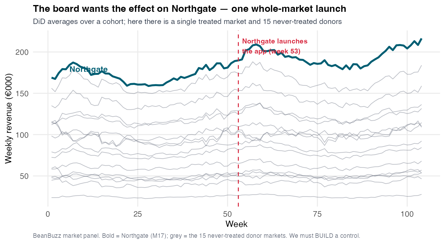
Log weekly revenue over 104 weeks. One bold line is Northgate, the largest BeanBuzz market, sitting visibly above a fan of fifteen thin grey never-treated donor markets. A vertical line marks go-live at week 53, after which the bold Northgate line pulls further above the grey band.

S10 answered “what’s the app worth on average?” The board now asks a different question: what did it do to Northgate — our flagship, market M17, the largest, seven stores, go-live week 53.

One treated unit breaks the DiD machinery

DiD needed a cohort — many units launched at similar times, so parallel trends could lean on an average and a comparison pool.

Northgate is one unit. Its pre-trend is mostly noise; there is no cohort to average over.

The single-unit problem

With one treated market and no cohort, “do the treated and controls move in parallel?” has nothing to discipline it. We need a different way to build the counterfactual.

To be clear, the number is not the problem: a plain 2×2 DiD on Northgate already gives +7.7% (true +8.3%). What fails at N = 1 is defending it — no cohort, no clustered inference, no pre-test power.

A weighted control is a synthetic unit

DiD and synthetic control differ in one choice — the donor weights. That flips the direction the missing \(Y(0)\) is imputed from:

  • DiD: every clean control gets weight 1. It projects the treated unit forward in time on the donors’ common trend — a horizontal borrow.
  • Synthetic control: solve for a convex blend \(\omega\) (non-negative, summing to 1) that tracks the treated unit pre-launch. Each missing cell is a weighted column of donors — a vertical borrow.

The blend is a synthetic Northgate — a fictional market from real donors, standing in for the one we can’t observe.
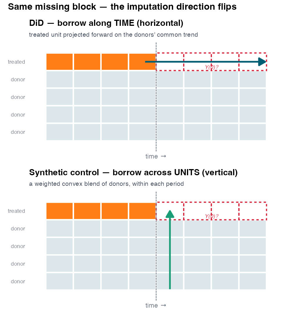
Two stacked units-by-time grids for the same panel. In both, the treated unit is the top row (orange pre-treatment cells) and its post-treatment cells form a red-dashed missing Y(0) block. Top panel (DiD): a horizontal arrow runs along the treated row into the missing block — imputing along time from the common trend. Bottom panel (synthetic control): a vertical arrow runs up a post-treatment column from the donor rows into the treated missing cell — imputing across units from a weighted blend of donors.

Building a Synthetic Unit

Match the pre-period, not the covariates alone

Abadie-Diamond-Hainmueller’s objective: choose donor weights \(\omega\) to make the synthetic unit’s pre-treatment outcome path track the treated unit’s. (Abadie, Diamond, and Hainmueller 2010)

\[\min_{\omega}\ \sum_{t \le T_0}\Big(Y^{\text{treat}}_t - \sum_{j}\omega_j\,Y^{\text{donor}}_{j,t}\Big)^2 \quad \text{s.t. } \omega_j \ge 0,\ \textstyle\sum_j \omega_j = 1\]

The constraints make \(\omega\) a point in the simplex — non-negative, summing to 1. Convexity = no extrapolation: the synthetic unit stays inside the donors’ range.

California’s tobacco tax: the textbook fit
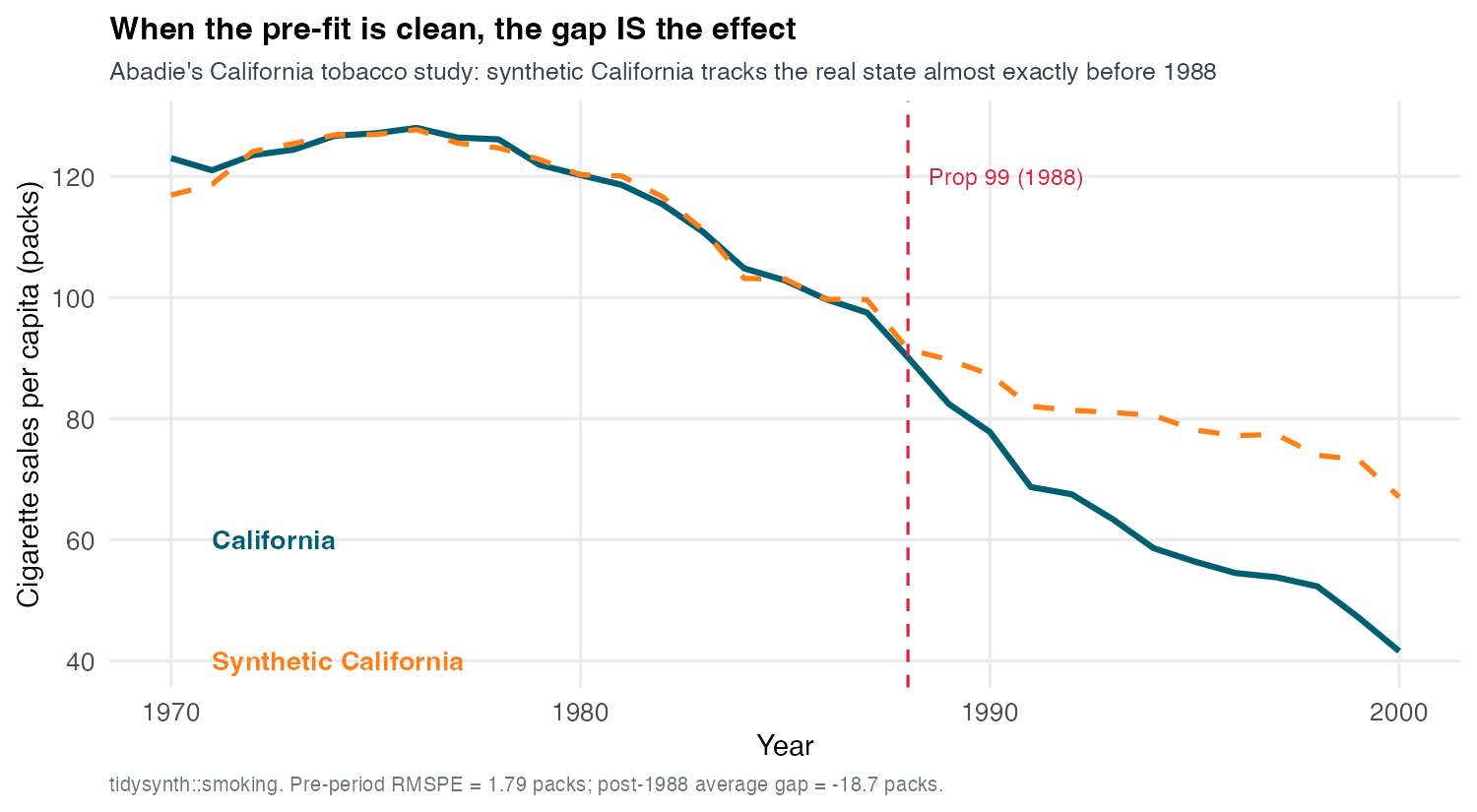
Per-capita cigarette sales from 1970 to 2000 for California (solid) and a synthetic California built from a weighted blend of other states (dashed). Before 1988 the two lines lie almost on top of each other. A vertical line marks Proposition 99 in 1988, after which the solid California line drops below the dashed synthetic line.

Abadie’s original case: California’s Proposition 99 (1988). Synthetic California — a blend of other states — tracks the real state almost exactly before the tax (pre-RMSPE ≈ 1.8 packs). (Abadie, Diamond, and Hainmueller 2010, 2015)

The gap plot reads the treatment effect off
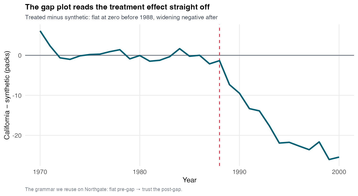
The gap between real and synthetic California per-capita cigarette sales over time. Before 1988 the gap hovers tightly around zero. After the 1988 Proposition 99 line, the gap opens steadily downward, reaching about minus 18.7 cigarettes per capita by the late 1990s.

Subtract synthetic from real and plot the gap. Flat at zero before 1988 (the fit was clean); it opens to ≈ −18.7 cigarettes/capita after — the effect of the tax.

Northgate doesn’t fit as cleanly as California
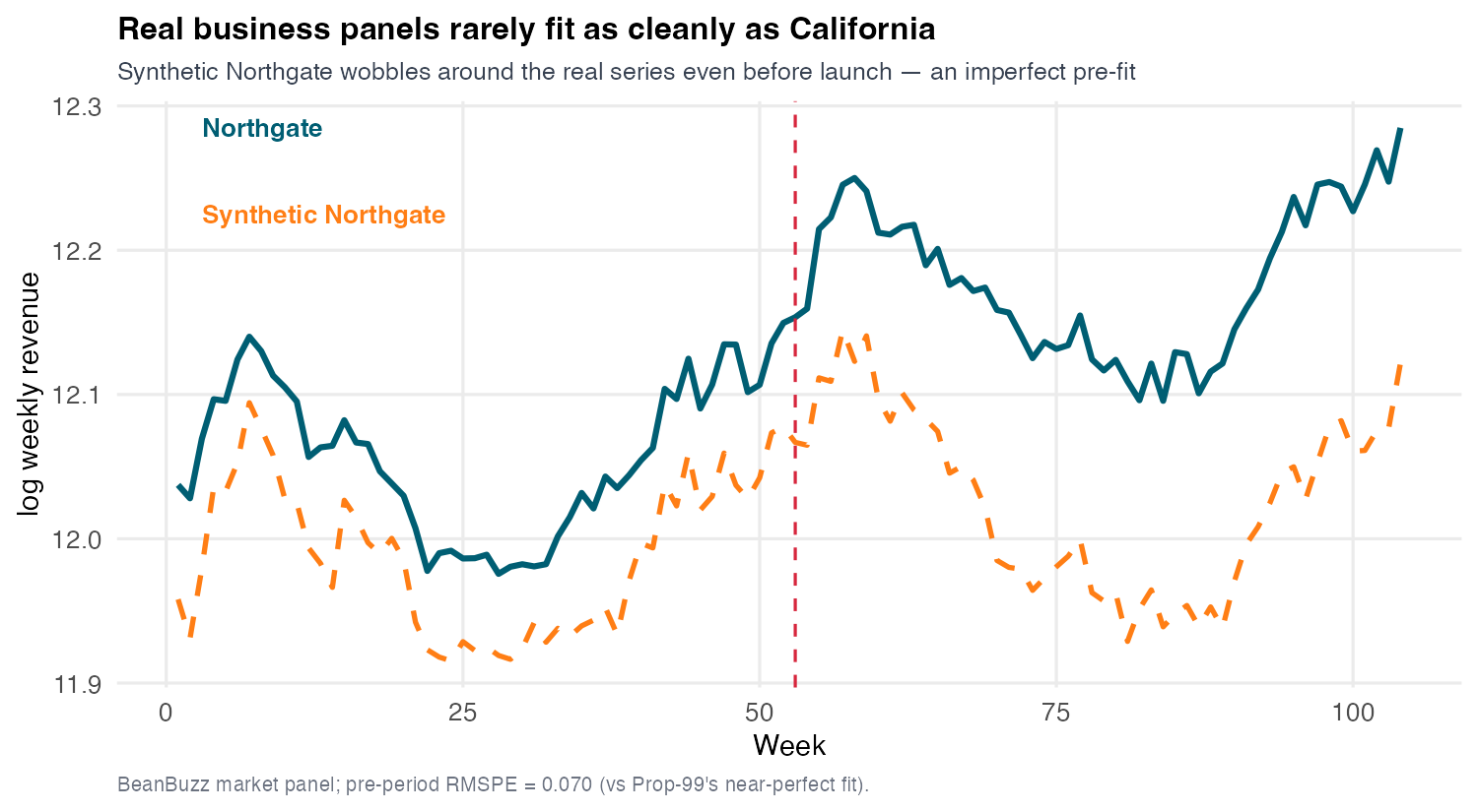
Log weekly revenue for Northgate (solid) and its classic synthetic control (dashed) over 104 weeks. Before the week 53 launch line the synthetic line sits visibly below the solid Northgate line rather than on top of it — a persistent gap. After launch the solid line pulls even further above the dashed one.

Same recipe, harder unit. Northgate is the largest market — at the edge of the donor convex hull. No blend of smaller donors reaches its level: the dashed synthetic sits persistently below before launch.

An imperfect pre-fit inflates the estimate
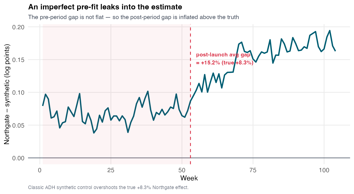
The gap between Northgate and its classic synthetic control over time. Before the week 53 launch the gap sits well above zero at roughly plus 6.8 percent rather than flat at zero. After launch the gap rises further to about plus 15.2 percent. The non-flat pre-period is annotated as a baked-in offset.

The pre-gap isn’t flat — it sits at +6.8% (pre-RMSPE ≈ 0.070). That offset leaks straight into the post-gap:

+15.2% ≈ pre-offset +6.8% + true effect +8.3%

Read the weights: which markets, how much
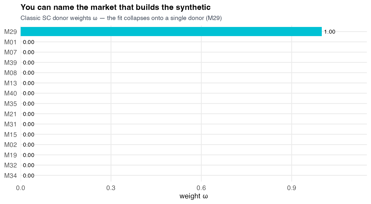
A bar chart of classic synthetic-control unit weights across the fifteen donor markets. One donor, M29, receives essentially all the weight (about 1.00) while every other market sits at zero, so the synthetic Northgate is built from a single market.

The blend is maximally sparse — one donor (M29) carries essentially all the weight, the rest sit at zero. That single weight vector is still a row describing how to rebuild one unit from the others (a seed for the matrix view later).

Donor hygiene decides what the weights can mean

A synthetic unit is only as good as its donor pool. Three hygiene rules:

  • Convex hull. The treated unit must be spannable by donors. Northgate barely is — that’s the +6.8% offset.
  • Plausible donors. Drop markets that are structurally unlike the treated unit; a good numerical fit on irrelevant donors is a mirage.
  • No spillover (SUTVA). A donor contaminated by the treatment (e.g. a neighbour that also adopted) is not a clean control. (O’Riordan 2025; Di Stefano-Mellace 2024)

Inference

No standard error — so permute the donors

Is +15.2% distinguishable from noise? With one treated market and one realized path, there is no sampling distribution — no classic standard error. Abadie’s answer is a randomization test. (Abadie, Diamond, and Hainmueller 2010, 2015)

Placebo-in-space, three steps:

  1. Reassign treatment to each donor in turn (fake launch, week 53); re-run synthetic control → its gap path.
  2. Score each unit by its MSPE ratio — post-period ÷ pre-period mean-squared gap.
  3. Rank by that ratio: Northgate’s rank ÷ number of units = the Fisher p-value.

Why the ratio, not the raw gap

MSPE = the mean squared gap between a unit and its synthetic. Dividing post ÷ pre asks whether the gap grew after treatment relative to the pre-fit — so a placebo whose synthetic never tracked it can’t top the ranking just by being noisy.

Northgate’s gap stands out — but not overwhelmingly
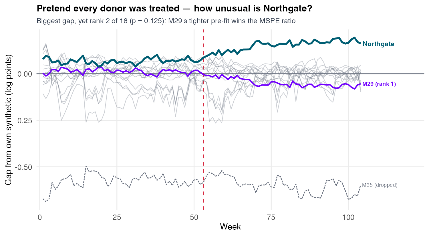
A fan of fifteen placebo gap paths, one per donor market, across 104 weeks. Northgate's path (bold teal) opens upward after week 53 to the largest gap. One donor, M29 (purple), is highlighted near zero and labelled rank 1 — its near-perfect pre-fit gives it a higher MSPE ratio than Northgate despite a tiny gap. A second donor, M35 (grey dashed near minus 0.6), is labelled dropped: its poor pre-fit removes it under the fit-filter.

Northgate’s gap is the biggest, yet it ranks 2 of 16 (Fisher p = 0.125; fit-filtered 2 of 15, p = 0.133). The test scores by MSPE ratio (post ÷ pre), so M29’s near-perfect pre-fit outranks Northgate’s bigger-but-noisier gap — not a larger effect.

Honest reading: with 15 donors and an imperfect fit, single-unit SC inference is fragile. Corroborate across methods — don’t hang the decision on one p-value.

Modern SC ships a real prediction interval

The placebo test asks “is it extreme?” Newer theory asks the sharper question: how uncertain is the counterfactual itself? (Cattaneo et al. 2025)

The synthetic counterfactual is \(\widehat{Y}^{(0)}_t=\sum_{j}\widehat{\omega}_j\,Y_{jt}\). Its prediction error has two sources: in-sample — the weights \(\widehat{\omega}\) are estimated on a finite pre-period — and out-of-sample — irreducible noise in predicting a future path.

What scpi reports

A \((1-\alpha)\) prediction interval for the counterfactual \(Y^{(0)}_t\) — bounding the in-sample error and modelling the out-of-sample noise. Read the effect as \(\widehat{\tau}_t=Y^{\text{obs}}_t-\widehat{Y}^{(0)}_t\): the actual above the whole band means \(\tau_t>0\). A band for \(Y(0)\), not a sampling SE for the point.

Actual above the band → a positive effect
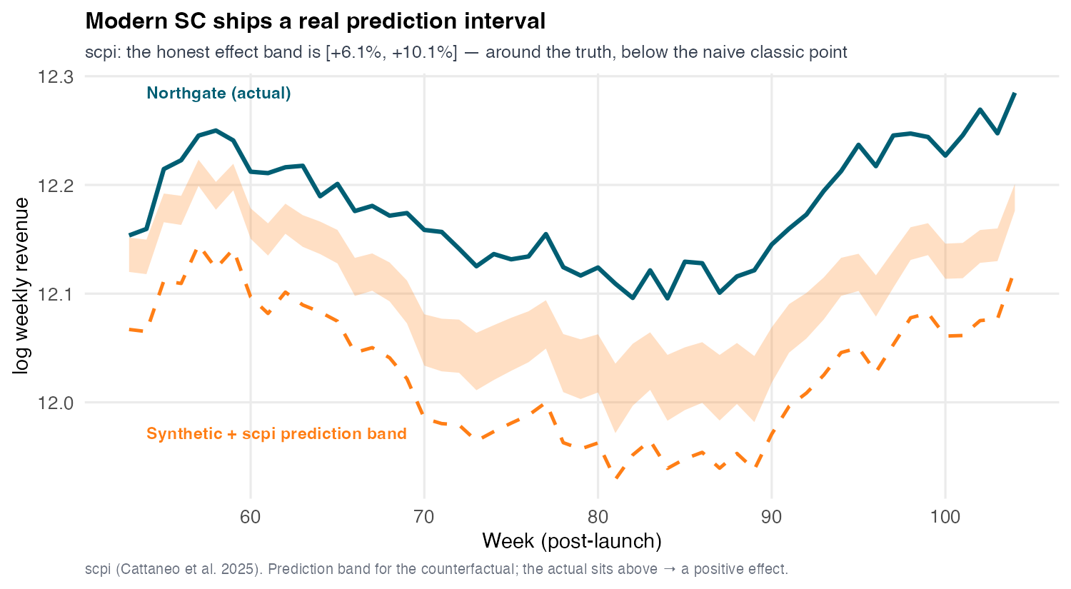
Northgate's actual log revenue path (solid teal) sits above the orange dashed synthetic counterfactual and its shaded orange scpi prediction band across the post-period. The gap between the actual and the band is the treatment effect; the implied effect band spans roughly plus 6.1 to plus 10.1 percent, below the naive plus 15 point estimate.

Orange dashed = the synthetic counterfactual \(\widehat{Y}^{(0)}\); orange band = its scpi prediction interval (for \(Y(0)\)); teal = Northgate’s actual path. The gap between them is the effect: the honest effect band is [+6.1%, +10.1%], near the true +8.3% and well below the naive ≈+15% point. The actual sits above the band → a positive effect, and the naive point was overconfident.

Augmented SC

If you can’t fit inside the hull, correct outside it

Northgate is outside the donors’ hull, so no convex blend reaches it — the +6.8% offset. Augmented SC adds a ridge outcome-model correction that steps outside the simplex just enough. (Ben-Michael, Feller, and Rothstein 2021)

  • SCM (classic SC) — on the hull boundary, the closest it can get.
  • Ridge ASCM (augmented) — steps outside toward the treated unit.
  • Uniform (DiD average) — deep inside; the path runs green (in simplex) → red (in hull) → blue (out of hull).
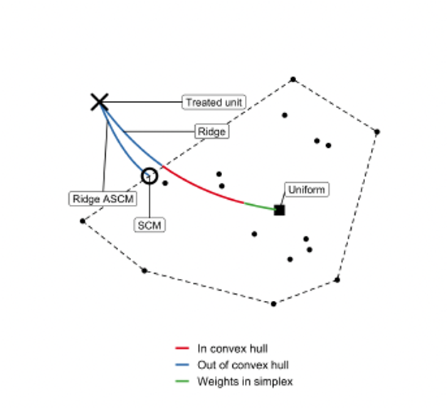
A schematic covariate space. Donor points form a dashed convex hull; the treated unit (X) lies outside it to the upper left. A path runs from the Uniform DiD average (black square inside the hull) out to the treated unit — coloured green while the weights are in the simplex, red while inside the convex hull, and blue once outside it. Classic SC (SCM) is where the path meets the hull boundary; ridge augmented SC (Ridge ASCM), circled, sits just outside the boundary toward the treated unit.

Source: Ben-Michael, Feller & Rothstein (2021)

Augmented SC = outcome model + residuals

Correct the classic weights’ leftover pre-period imbalance with an outcome model \(\widehat{m}(X)\): (Ben-Michael, Feller, and Rothstein 2021)

\[\begin{aligned} \widehat{Y}^{(0),\text{aug}}_{1T} &=\underbrace{\sum_i \widehat{\omega}^{sc}_i\,Y_{iT}}_{\text{classic SC}}+\underbrace{\Big(\widehat{m}(X_1)-\sum_i \widehat{\omega}^{sc}_i\,\widehat{m}(X_i)\Big)}_{\text{imbalance correction}}\\ &=\underbrace{\widehat{m}(X_1)}_{\text{outcome model}}+\underbrace{\sum_i \widehat{\omega}^{sc}_i\big(Y_{iT}-\widehat{m}(X_i)\big)}_{\text{SC-reweighted residuals}} \end{aligned}\]

  • Doubly robust: consistent if either the SC weights balance the pre-period or \(\widehat{m}\) is correct.
  • Ridge outcome model: \(\widehat{m}(X)=\widehat{\eta}_0+X'\widehat{\eta}_x\), penalty \(\lambda\) by CV — the weights may leave the simplex, the ridge curbs extrapolation.

Augmented SC pulls the overshoot toward truth
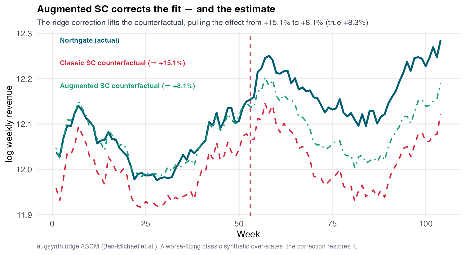
Two counterfactual paths for Northgate over 104 weeks. The classic synthetic control (red) sits persistently below the real path before week 53, leaving a baked-in offset. The augmented synthetic control (green) lies almost exactly on the real path before launch, closing the pre-period gap. After launch the two counterfactuals diverge, with the green one higher.

Closing the pre-fit (offset ≈ 0.000) collapses the overshoot: augmented SC = +8.1%, 95% CI [+7.6%, +8.6%] — essentially the true +8.3%. Classic +15.2% → augmented +8.1%.

Fit is a diagnostic, not a verdict

A great pre-fit feels like proof. It isn’t — fit is necessary, never sufficient.

The Ferman caution

Overfitting the pre-period ≠ an unbiased counterfactual. With many donors and a short pre-period you can drive the pre-fit to zero and still be biased — the weights fit noise, not structure. (Ferman and Pinto 2021)

So report three things, never one

  1. The fit — pre-period RMSPE / gap plot (necessary, not sufficient).
  2. An interval — scpi band or placebo p-value (how uncertain?).
  3. Cross-method agreement — do augmented / SDID / DiD concur?

This is the discipline S10 demanded — “corroborate with synthetic control.” The honesty rule: a point estimate without a band is not a finding.

Synthetic DiD

DiD weights time; SC weights units

The two methods we’ve used weight different axes of the same panel:

  • DiD weights time: it gives every clean control unit weight 1, and identifies off the common time trend (the period effects).
  • Synthetic control weights units: it solves for donor weights \(\omega\), and gives every pre-period equal weight.

Each fixes one axis and optimizes the other. The obvious question: why not weight both?

Synthetic DiD weights both axes

Arkhangelsky et al.’s synthetic difference-in-differences: solve for unit weights \(\omega\) and time weights \(\lambda\), then run a weighted two-way DiD — three corners of one family. (Arkhangelsky et al. 2021)
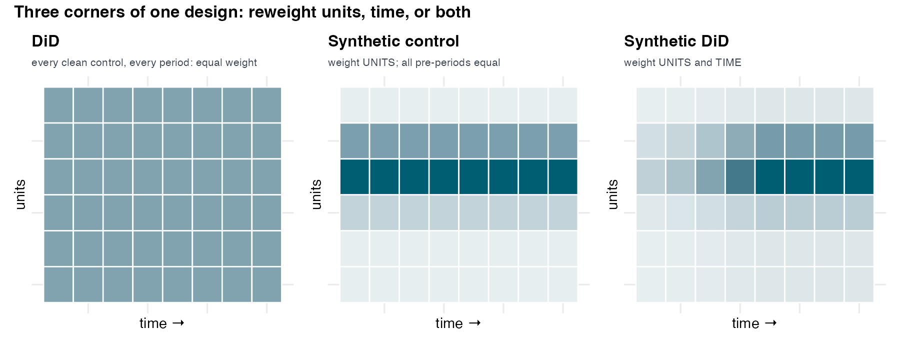
Three side-by-side unit-by-time weighting grids. The DiD grid weights all units equally and all times equally. The synthetic control grid concentrates weight on a few donor units but spreads it evenly across pre-periods. The synthetic DiD grid concentrates weight on both a few donor units and a few informative pre-periods.

Robust to both failure modes

  • \(\omega\) (like SC) matches donors to the treated unit → robust to non-parallel trends.
  • \(\lambda\) (new) up-weights pre-periods that resemble the post-period → robust to an imperfect pre-fit. It needs neither a perfect SC fit nor exact parallel trends.

DiD, SC, and SDID are one weighted regression

Synthetic DiD is a two-way fixed-effects regression with the squared errors reweighted by \(\widehat\omega_i\,\widehat\lambda_t\):

\[(\widehat\tau^{\,sdid},\widehat\mu,\widehat\alpha,\widehat\beta)=\arg\min_{\tau,\mu,\alpha,\beta}\ \sum_{i=1}^{N}\sum_{t=1}^{T}\big(Y_{it}-\mu-\alpha_i-\beta_t-D_{it}\,\tau\big)^2\,\widehat\omega_i\,\widehat\lambda_t\]

\(\mu\) intercept · \(\alpha_i\) unit (market) effects · \(\beta_t\) period (week) effects · \(D_{it}=1\) for the treated market post-launch · \(\tau\) the ATT

Estimator Unit FE (α) Weights on the squared errors
DiD yes uniform ω, uniform λ (drop out) → plain TWFE
SC omitted unit weights ω only; uniform λ
SDID yes both ω and λ

All three keep the period effects \(\beta_t\) — DiD’s “time” leverage (the common trend), not a time weight. They differ only in whether the unit FE \(\alpha_i\) is kept and which of the weights \(\omega,\lambda\) are non-uniform.

SDID lands near the truth on Northgate
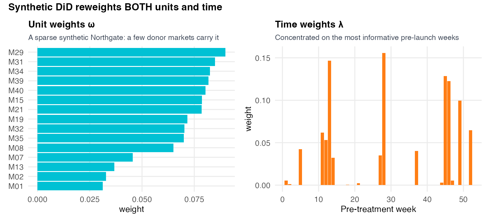
The synthetic difference-in-differences weight bars for Northgate: unit weights concentrated on a few donor markets on the left, time weights concentrated on a subset of pre-treatment weeks on the right.

Northgate’s unit and time weight vectors — now we know what they buy. Synthetic DiD = +7.9% (true +8.3%); plain DiD = +7.7%. Both near the truth, without a perfect SC fit.

Watch SDID stay parallel where classic SC drifts
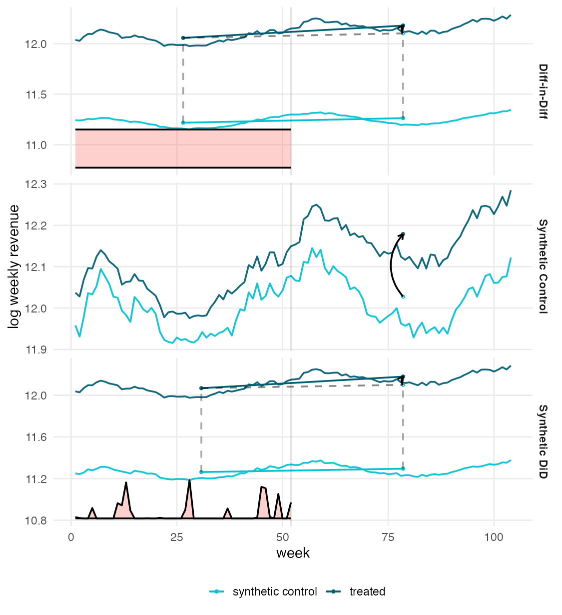
Three stacked panels — Diff-in-Diff, Synthetic Control, Synthetic DiD — each plotting treated Northgate (dark) against its synthetic control (cyan) over 104 weeks, with a treatment line at week 53, the estimated effect drawn as an arrow at the post end, and a shaded time-weight ribbon along the bottom.

Same three estimators as trajectories: treated Northgate (dark) vs its synthetic control (cyan); the effect is the arrow after week 53.

  • SDID (bottom): the \(\lambda\) ribbon marks the pre-weeks where the two lines are forced parallel → a short, well-anchored arrow (+7.9%).
  • Classic SC (middle): the synthetic can’t close the level gap → a longer arrow (the +15.2% overshoot).
  • DiD (top): matches the trend, not the level — it leans entirely on parallel trends.

That sparse \(\lambda\) ribbon is the same time-weight vector you saw as bars — now as the pre-window that makes the lines parallel.

The family converges on ~+8%; classic SC stands alone
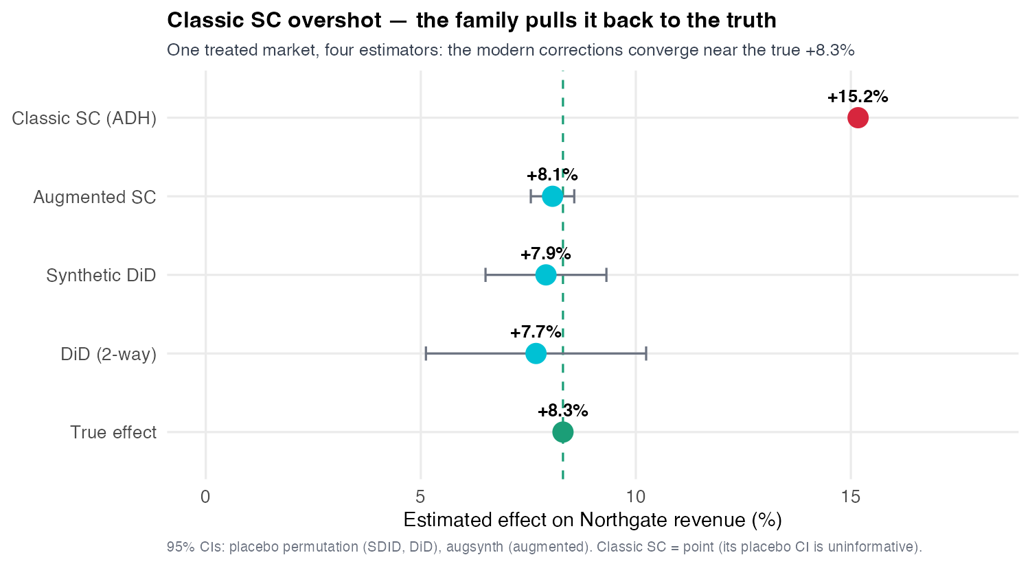
A forest plot of Northgate estimators against a dashed line at the true effect of plus 8.3 percent. Classic synthetic control is a bare point far to the right at plus 15.2. Augmented SC (plus 8.1), synthetic DiD (plus 7.9) and plain DiD (plus 7.7) cluster near the true line, each with a 95 percent confidence interval that contains it — augmented SC's tight, synthetic DiD's moderate, plain DiD's the widest; the classic point is the lone outlier with no interval shown.

Classic SC +15.2% is the lone outlier; augmented +8.1% · SDID +7.9% · DiD +7.7% all cluster on the true +8.3%.

Methods that fail in different ways agreeing is the verdict the single placebo p-value couldn’t give — the honest answer is ~+8% with a band, not fifteen.

Each method buys an assumption — stacked, they’re one matrix

Family What it buys What it costs
Parallel-trends family
S10 — DiD, CS, BJS
Additive, transparent, cheap; borrows strength across a whole cohort. Blind to a unit-specific, time-varying factor; needs a credible cohort and testable pre-trends.
Hull + loadings
S11 — SC, augmented SC, SDID
Relaxes parallel trends; builds a unit-specific counterfactual that works at N = 1. Needs the treated unit inside the donor hull and a non-overfit pre-fit; single-unit inference is weak.

The S12 reveal — planted here

Stack \(\omega\) and \(\lambda\) as rows and you’re completing a low-rank matrix — the same latent factors S10 could not see. S12: DiD, SC, SDID and unconfoundedness become one matrix-completion problem under different regularizers.

One treated unit was the easy case

Every estimator here weighted donors to build a counterfactual for one unit at one adoption date. Scale that up and the weighting paradigm answers by multiplying bookkeeping.

Many units — one date

A synthetic control per unit (then average), or one fit to their average? The honest default is partial pooling — a dial between the two.

Staggered dates

Split into adoption cohorts, solve an N = 1 fit per cohort in event time, then aggregate — SC’s Callaway–Sant’Anna analog, with one rule: never borrow from an already-treated unit.

Why S12 exists

This scales by adding bookkeeping — and still can’t represent a unit switching off. Impute the whole \(Y(0)\) matrix instead: matrix completion fills every grey cell from one low-rank structure, absorbing many units, staggered timing, and reversal natively.

References

Abadie, Alberto, Alexis Diamond, and Jens Hainmueller. 2010. “Synthetic Control Methods for Comparative Case Studies: Estimating the Effect of California’s Tobacco Control Program.” Journal of the American Statistical Association 105 (490): 493–505. https://doi.org/10.1198/jasa.2009.ap08746.
———. 2015. “Comparative Politics and the Synthetic Control Method.” American Journal of Political Science 59 (2): 495–510. https://doi.org/10.1111/ajps.12116.
Arkhangelsky, Dmitry, Susan Athey, David A. Hirshberg, Guido W. Imbens, and Stefan Wager. 2021. “Synthetic Difference-in-Differences.” American Economic Review 111 (12): 4088–118. https://doi.org/10.1257/aer.20190159.
Ben-Michael, Eli, Avi Feller, and Jesse Rothstein. 2021. “The Augmented Synthetic Control Method.” Journal of the American Statistical Association 116 (536): 1789–1803. https://doi.org/10.1080/01621459.2021.1929245.
Cattaneo, Matias D., Yingjie Feng, Filippo Palomba, and Rocío Titiunik. 2025. “Scpi: Uncertainty Quantification for Synthetic Control Methods.” Journal of Statistical Software 113 (1): 1–38. https://doi.org/10.18637/jss.v113.i01.
Chernozhukov, Victor, Kaspar Wüthrich, and Yinchu Zhu. 2021. “An Exact and Robust Conformal Inference Method for Counterfactual and Synthetic Controls.” Journal of the American Statistical Association 116 (536): 1849–64. https://doi.org/10.1080/01621459.2021.1920957.
Ferman, Bruno, and Cristine Pinto. 2021. “Synthetic Controls with Imperfect Pretreatment Fit.” Quantitative Economics 12 (4): 1197–1221. https://doi.org/10.3982/QE1596.
Thank you for your attention!