library(readr); library(dplyr); library(ranger); library(fixest)
covars <- c("age","gender","region","prior_courses",
            "baseline_score","device","track")
set.seed(42)
df <- read_csv(here::here("materials/data/learnloop_dml.csv"), show_col_types = FALSE) |>
  mutate(across(c(gender, region, device, track), as.factor))

# (a) Contrasts: how far off are the naive and the linear-controls OLS?
# ___ YOUR CODE: feols(exam_score ~ recommended, df)              # naive
# ___ YOUR CODE: feols(exam_score ~ recommended + age + gender + region + prior_courses + baseline_score + device + track, df)  # linear adj.

# (b) 5-fold cross-fit  l_hat = E[Y|X]  and  m_hat = E[D|X]  with ranger (mtry = 4!)
n <- nrow(df); n_folds <- 5
folds <- sample(rep(1:n_folds, length.out = n))
Y <- df$exam_score; D <- df$recommended; Xdf <- df[, covars]
l_hat <- m_hat <- numeric(n)
for (k in 1:n_folds) {
  tr <- folds != k; te <- folds == k
  # ___ YOUR CODE: fitY <- ranger(x = Xdf[tr, ], y = Y[tr], num.trees = 500, mtry = 4); fitD <- same on D[tr]
  # ___ YOUR CODE: l_hat[te] <- predict(fitY, Xdf[te, ])$predictions; m_hat[te] <- predict(fitD, Xdf[te, ])$predictions
}

# (c) Residualize and solve the partialling-out moment
# ___ YOUR CODE: res_y <- Y - l_hat ; res_d <- D - m_hat
# ___ YOUR CODE: tau_plr <- sum(res_y * res_d) / sum(res_d^2)

# (d) Influence-function SE and a 95% CI — does it cover 5.0?
# ___ YOUR CODE12 Session 8: Double Machine Learning
12.1 Lecture Slides
12.2 Overview
This session returns to the world of S06 — selection on observables, where conditioning on a covariate set \(\mathbf{X}\) makes treatment as-good-as-random — but with a complication S06 could not handle: \(\mathbf{X}\) is high-dimensional and the confounding runs through nonlinear interactions that no hand-specified linear control can absorb. The natural impulse is to throw a flexible machine learner at the nuisance functions \(E[Y\mid\mathbf{X}]\) and \(E[D\mid\mathbf{X}]\). The catch is that a machine that predicts well is not a machine that estimates well: a naive plug-in inherits the learner’s slow convergence rate and two distinct biases — regularization bias (shrinkage that leaks into the treatment coefficient) and overfitting bias (a model evaluated on its own training rows). Double Machine Learning (DML) is the bookkeeping that turns flexible nuisance predictions into a valid causal estimate with an honest confidence interval. It does so with exactly two ingredients — a Neyman-orthogonal score that kills regularization bias and cross-fitting that kills overfitting bias — wrapped in a single four-step recipe that instantiates on two core models (the partially linear model and the AIPW/interactive model) plus two instrumental-variable variants (partially linear IV and interactive IV). Throughout we estimate average effects (ATE, LATE); the per-unit score we build here is the object that next week’s heterogeneity methods will project rather than average.
Key takeaways
- DML = Frisch–Waugh–Lovell with a machine. Partial \(\mathbf{X}\) out of both \(Y\) and \(D\) using any ML learner, then read the residual-on-residual slope. The only role of \(\mathbf{X}\) is to be partialled out.
- Two ingredients restore valid inference. Orthogonality makes the estimate first-order insensitive to nuisance error (bias becomes the product of two errors, not their sum); cross-fitting decouples nuisance estimation from the moment that estimates \(\tau\). Neither alone suffices — only both together recover the \(\sqrt{n}\), asymptotically normal sampling distribution.
- One recipe, two models, plus DML-IV. Switch only the score and you switch the estimand: the partially linear model (constant \(\tau\)), the AIPW/interactive model (doubly-robust ATE), and the interactive IV model (LATE on compliers). Steps 2–4 — cross-fit, solve the moment, read the influence-function SE — never change.
- DML solves estimation, not identification. It buys freedom from specifying the functional form of the nuisances; it does nothing about an unobserved confounder. Unconfoundedness remains an untestable assumption, so always stress-test the estimate with a sensitivity analysis.
12.3 Lecture Notes
12.3.1 A machine that predicts is not a machine that explains
12.3.1.1 The deliverable is a number and a trustworthy interval
The output of a causal analysis is not a point estimate but a point estimate equipped with calibrated uncertainty. Formally, we want an estimator \(\hat\tau\) of the target effect \(\tau\) whose sampling distribution satisfies
\[\sqrt{n}\,(\hat\tau - \tau) \;\xrightarrow{d}\; \mathcal{N}(0, V),\]
because that single line is what licenses the everyday confidence interval \(\hat\tau \pm 1.96\,\widehat{\text{SE}}\). It demands three things at once: consistency (\(\hat\tau \to \tau\), we hit the target), the \(\sqrt{n}\) rate (the error shrinks fast enough that the interval is informative at realistic sample sizes), and asymptotic normality (so the \(1.96\) multiplier delivers genuine 95% coverage). A learner chosen to minimise prediction error on \(Y\) optimises none of these for \(\tau\). It can predict exam scores with a small test error and still return a treatment-effect estimate that is biased, wrongly scaled, and attached to a confidence interval that under-covers. Everything in this session is in service of recovering that one display line while letting machine learning do the heavy lifting on the nuisances.
12.3.1.2 Two biases, and the \(n^{-1/4}\) rate that dooms the naive plug-in
Plug a flexible learner \(\hat g(\mathbf{X})\) into a naive estimator of \(\tau\) and two biases leak in. Regularization bias: every good ML method trades variance for bias by shrinking — the lasso penalty, shallow trees, early stopping — and because the treatment \(D\) is itself related to \(\mathbf{X}\), that shrinkage is correlated with \(D\) and contaminates \(\hat\tau\) directly (Figure 12.1). Overfitting bias: if the same rows that train the nuisance also enter the moment that estimates \(\tau\), the model has partly memorised its own noise, which biases the point estimate and, just as damagingly, shrinks the estimated standard error so the interval under-covers.
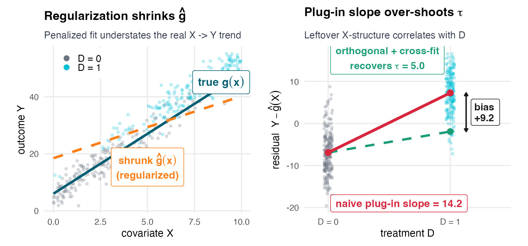
The deeper problem is the rate. Nonparametric ML nuisances typically converge at \(n^{-1/4}\) — far slower than the parametric \(n^{-1/2}\). A naive plug-in passes this slow rate straight through to \(\tau\): its bias is \(O(n^{-1/4})\), so \(\sqrt{n}\,(\hat\tau - \tau) \sim \sqrt{n}\cdot n^{-1/4} = n^{1/4} \to \infty\). The standardized estimator diverges; the confidence interval is worthless. The entire trick of DML is to construct a score whose bias depends not on a single \(n^{-1/4}\) error but on the product of two of them — \(n^{-1/4}\cdot n^{-1/4} = n^{-1/2}\) — which is exactly fast enough to vanish under \(\sqrt{n}\) scaling (Chernozhukov et al. 2018).
12.3.1.3 LearnLoop: does the recommender actually lift exam scores?
The running example is LearnLoop, an online-learning platform whose recommender suggests the next module \(D=\texttt{recommended}\) (binary) and measures the next-period exam score \(Y=\texttt{exam\_score}\). The observed covariates \(\mathbf{X}\) are age, gender, region, prior_courses, baseline_score, device, and track. A naive comparison of treated and untreated learners reports a lift of \(\approx 14.03\) points — but the recommender deliberately targets stronger learners, who would have scored higher anyway. The lift is confounded by \(\mathbf{X}\), and crucially the confounding runs through a nonlinear interaction (baseline_score \(\times\) prior_courses) that a linear control cannot represent. Tossing the covariates into an additive linear regression moves the estimate to \(\approx 5.47\) — much closer, but its confidence interval still excludes the truth, because the model cannot see the interaction. The synthetic data are constructed so the true ATE is \(5.0\), which lets us check every number we compute. DML, by residualizing with a learner that captures the interaction, lands on \(\approx 5.0\).
12.3.1.4 The whole session in one recipe
Two ingredients do the real work: orthogonality (kills regularization bias, Neyman orthogonality) and cross-fitting (kills overfitting bias, cross-fitting). Acts 2–3 build the two ingredients; Act 4 runs the recipe on two models (PLR and AIPW); Act 5 adds a third nuisance for the IV case; Act 6 stress-tests the identifying assumption. The only thing that changes across models is the score in step 1.
12.3.2 Partialling-out: from FWL to Robinson
12.3.2.1 Frisch–Waugh–Lovell — you already know the trick
To recover the coefficient on \(D\) in the regression \(Y \sim D + \mathbf{X}\), you do not need to run the full multivariate regression. The Frisch–Waugh–Lovell (FWL) theorem says that coefficient equals the slope of a residual-on-residual regression (Frisch and Waugh 1933; Lovell 1963):
- Regress \(Y\) on \(\mathbf{X}\); keep the residuals \(\tilde Y = Y - \hat{E}[Y\mid\mathbf{X}]\).
- Regress \(D\) on \(\mathbf{X}\); keep the residuals \(\tilde D = D - \hat{E}[D\mid\mathbf{X}]\).
- Regress \(\tilde Y\) on \(\tilde D\) — that slope is \(\hat\tau\), numerically identical to the full-OLS coefficient.
The reframing that opens the door to DML: the only role of \(\mathbf{X}\) in estimating \(\tau\) is to be partialled out of both \(Y\) and \(D\). OLS partials out by a linear projection, but nothing in FWL requires linearity. If \(E[Y\mid\mathbf{X}]\) and \(E[D\mid\mathbf{X}]\) are nonlinear, we may estimate them with any learner that captures that nonlinearity, and the residual-on-residual logic is preserved intact. This is the gentlest possible on-ramp to DML: it is FWL with a better residualizer. We have leaned on this same partialling-out idea before — matching in S06, and the 2SLS purge of \(D\) in S07.
12.3.2.2 Target versus nuisance: do not interpret every coefficient
This split is liberating. We are released from the regression-course habit of giving every coefficient a story. We no longer need a correct, interpretable model of \(g\); we need only to predict it well enough to partial it out. That is precisely the task at which machine learning excels, and it is exactly why we may hand \(g\) to a black box without guilt. It also foreshadows double robustness (the AIPW score): because \(g\) is a nuisance judged only by predictive quality, the right (orthogonal) score lets us be wrong about it in ways that do not contaminate \(\tau\).
12.3.2.3 The partially linear model (Robinson, 1988)
The partially linear regression (PLR) model formalises the split (Robinson 1988):
\[Y = \tau\, D + g(\mathbf{X}) + \varepsilon, \qquad \mathbb{E}[\varepsilon \mid D, \mathbf{X}] = 0,\] \[D = m(\mathbf{X}) + \nu, \qquad \mathbb{E}[\nu \mid \mathbf{X}] = 0.\]
The treatment enters linearly through a single number \(\tau\) — the constant treatment effect, here the ATE — while the controls enter arbitrarily through the two nuisance functions \(g(\mathbf{X})\) (the structural outcome function) and \(m(\mathbf{X}) = e(\mathbf{X}) = \mathbb{E}[D\mid\mathbf{X}]\) (the propensity). To derive the estimand, take the conditional expectation of the outcome equation given \(\mathbf{X}\). Because \(\mathbb{E}[\varepsilon\mid\mathbf{X}] = 0\) and \(\mathbb{E}[D\mid\mathbf{X}] = m(\mathbf{X})\),
\[\mathbb{E}[Y\mid\mathbf{X}] = \tau\, m(\mathbf{X}) + g(\mathbf{X}) \;\equiv\; \ell(\mathbf{X}).\]
Subtracting this line from the outcome equation cancels the \(g\) term entirely:
\[Y - \ell(\mathbf{X}) = \tau\,\bigl(D - m(\mathbf{X})\bigr) + \varepsilon, \qquad\text{i.e.}\qquad \tilde Y = \tau\,\tilde D + \varepsilon.\]
A population least-squares projection of \(\tilde Y\) on \(\tilde D\) then yields the partialling-out estimand
\[\tau = \frac{\operatorname{Cov}(\tilde Y, \tilde D)}{\operatorname{Var}(\tilde D)}, \qquad \tilde Y = Y - \ell(\mathbf{X}), \quad \tilde D = D - m(\mathbf{X}).\]
12.3.2.4 The leap, and LearnLoop in one figure
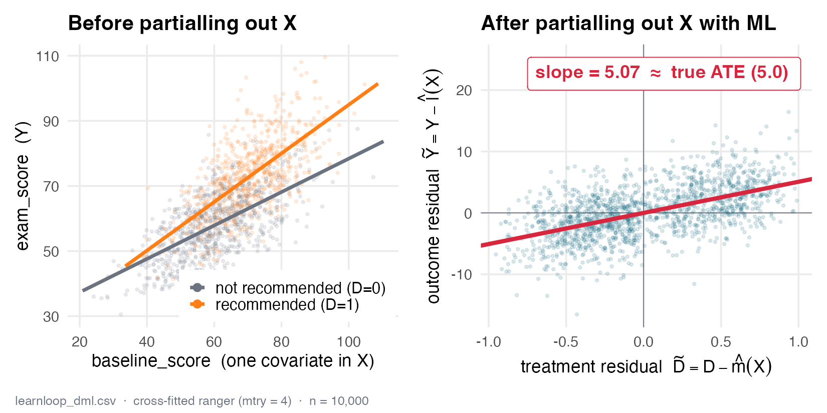
In LearnLoop terms, \(\tilde Y\) is the exam score with the part predictable from who the learner is removed, and \(\tilde D\) is the recommendation with that same predictable part removed — the as-good-as-random slice of treatment that remains once \(\mathbf{X}\) is accounted for. The slope of one residual on the other is the treatment effect, purged of \(\mathbf{X}\). Because the two partialling-out regressions are nothing but conditional-expectation estimates, we are free to estimate them with a random forest, lasso, gradient boosting, or a neural net instead of OLS. A linear residualizer can only remove linear/additive confounding; a flexible learner removes whatever structure is present. The LearnLoop confounding hides in a baseline_score \(\times\) prior_courses interaction — invisible to linear adjustment (which lands at \(\approx 5.47\)), visible to a forest (which snaps the residual-on-residual slope onto \(\approx 5.0\)). Run on LearnLoop, the two partialling-out regressions make the leap concrete (Figure 12.2).
12.3.3 Two ingredients: orthogonality + cross-fitting
12.3.3.1 Neyman orthogonality, stated precisely
The score (or moment function) \(\psi(W; \tau, \eta)\) is a function of the data \(W = (Y, D, \mathbf{X})\), the target \(\tau\), and the nuisance parameter \(\eta = (\ell, m)\). An estimator is defined by solving the empirical analogue of the moment condition
\[\mathbb{E}\bigl[\psi(W; \tau_0, \eta_0)\bigr] = 0,\]
which holds at the true parameter \(\tau_0\) and true nuisances \(\eta_0\). The danger is that in practice we plug in estimated nuisances \(\hat\eta \neq \eta_0\), and the resulting error in \(\hat\tau\) depends on how steeply the moment responds to perturbations of \(\eta\).
One structural fact makes the whole engine turn: every score in this session is linear in the target, \(\psi = \psi_a(W;\eta)\,\tau + \psi_b(W;\eta)\), so its root is closed-form, \[\hat\tau = -\,\frac{\mathbb{E}_n[\psi_b]}{\mathbb{E}_n[\psi_a]}\qquad(\text{cross-fitted } \hat\eta \text{ plugged in}).\] For the Robinson partialling-out score this reads \(\psi_a = -\tilde D^2\), \(\psi_b = \tilde Y\tilde D\), recovering the \(\operatorname{Cov}(\tilde Y,\tilde D)/\operatorname{Var}(\tilde D)\) slope of the partially linear model — and these are exactly DoubleML’s internal \(\psi_a, \psi_b\). The point is leverage: a single crank serves every model below (PLR, AIPW, IV), and only the score \(\psi\) changes.
To see why this is exactly what we need, compare two scores for the partially linear model.
The naive plug-in score. Suppose we estimate \(\hat g\) and use \(\psi^{\text{naive}} = (Y - \tau D - g(\mathbf{X}))\,D\). Perturb the outcome nuisance by \(g \to g + r\,\Delta_g\). Then \(\partial_r \mathbb{E}[\psi^{\text{naive}}]|_{r=0} = -\mathbb{E}[\Delta_g(\mathbf{X})\,D] \neq 0\) in general, because \(D\) is correlated with \(\mathbf{X}\) and hence with \(\Delta_g\). The first-order sensitivity is non-zero: a small error in \(\hat g\) produces a proportional error in \(\hat\tau\). This is regularization bias, formalised.
The orthogonal partialling-out (Robinson) score. Write it in residual form, \[\psi(W; \tau, \eta) = \bigl(\tilde Y - \tau\,\tilde D\bigr)\,\tilde D = \bigl(Y - \ell(\mathbf{X}) - \tau(D - m(\mathbf{X}))\bigr)\bigl(D - m(\mathbf{X})\bigr).\] Differentiating its expectation with respect to \(\ell\) in any direction \(\Delta_\ell\) gives \(-\mathbb{E}[\Delta_\ell(\mathbf{X})\,\tilde D] = -\mathbb{E}[\Delta_\ell(\mathbf{X})\,\nu] = 0\), because \(\nu = D - m(\mathbf{X})\) is mean-zero given \(\mathbf{X}\) and \(\Delta_\ell\) is a function of \(\mathbf{X}\) alone. Differentiating with respect to \(m\) gives a term proportional to \(\mathbb{E}[\varepsilon \mid \mathbf{X}] = 0\) at the truth. Both Gateaux derivatives vanish: the residualized score is Neyman-orthogonal. This is no accident — partialling out \(\mathbf{X}\) from both \(Y\) and \(D\) is precisely what centres the residuals so that the cross-terms with nuisance error drop out.
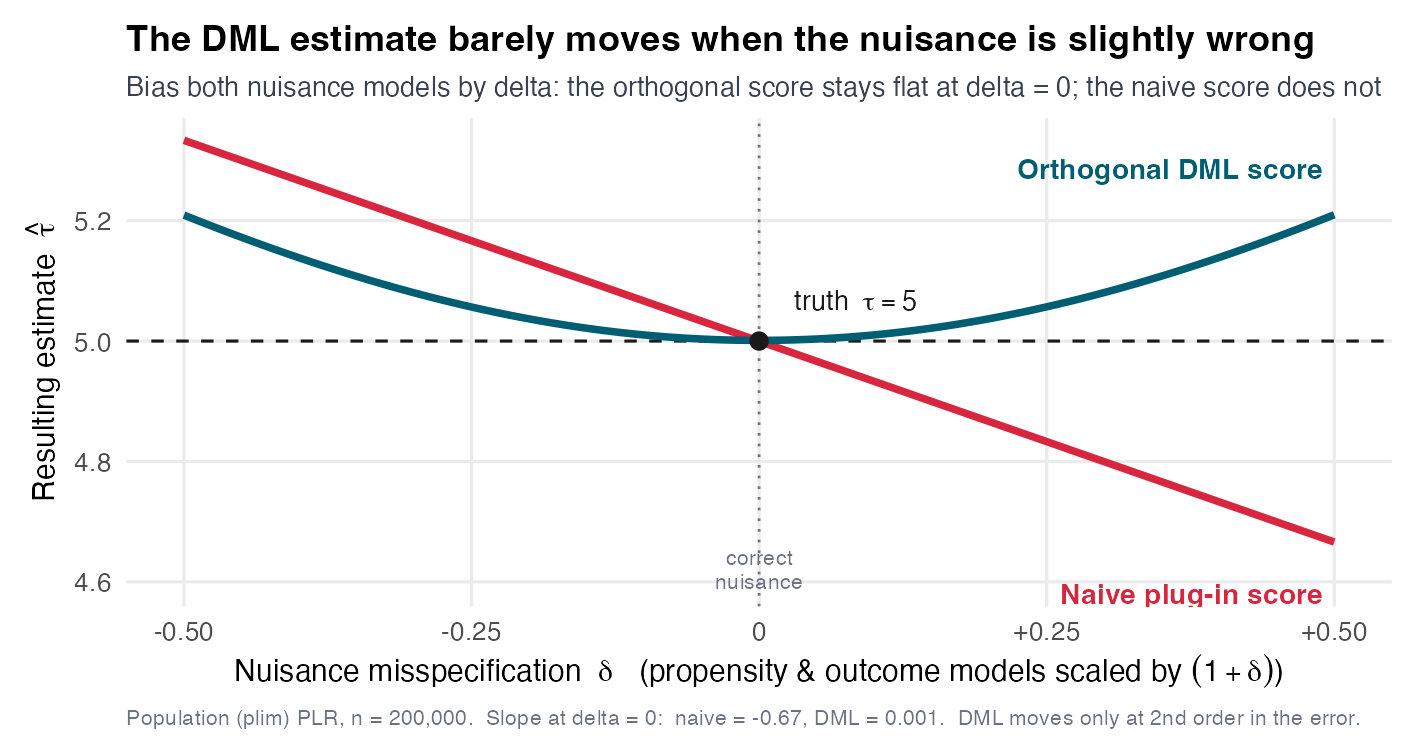
The payoff is the product-of-errors bias structure. For an orthogonal score the leading bias in \(\hat\tau\) is of the order \(\|\hat\ell - \ell_0\| \cdot \|\hat m - m_0\|\) — the product of the two nuisance errors, not their sum. If each ML nuisance converges at the typical \(n^{-1/4}\) rate, the product is \(n^{-1/2}\): fast enough for \(\sqrt{n}\,(\hat\tau - \tau)\) to remain stable and asymptotically normal. The figure below makes this visual (Figure 12.3): perturbing the nuisances by an amount \(\delta\) moves the naive plug-in along a line through the truth with a real slope, while the orthogonal score sits at the flat bottom of a parabola — its slope at \(\delta = 0\) is zero, so small nuisance errors cost essentially nothing.
12.3.3.2 Cross-fitting: never predict a unit with a model trained on it
Orthogonality alone is not sufficient. Even with an orthogonal score, if the same rows train the nuisance and enter the moment for \(\tau\), the model has seen its own noise, which reintroduces bias and — by making the in-sample fit look too good — shrinks the estimated standard error so that confidence intervals under-cover.
The fix is cross-fitting. Partition the sample into \(K\) folds. For each fold \(k\), fit the nuisances \(\hat\ell^{(-k)}, \hat m^{(-k)}\) on the other \(K-1\) folds, then form predictions only for the held-out fold \(k\). Rotating through all folds produces an out-of-fold prediction for every unit, each from a model that never saw that unit:
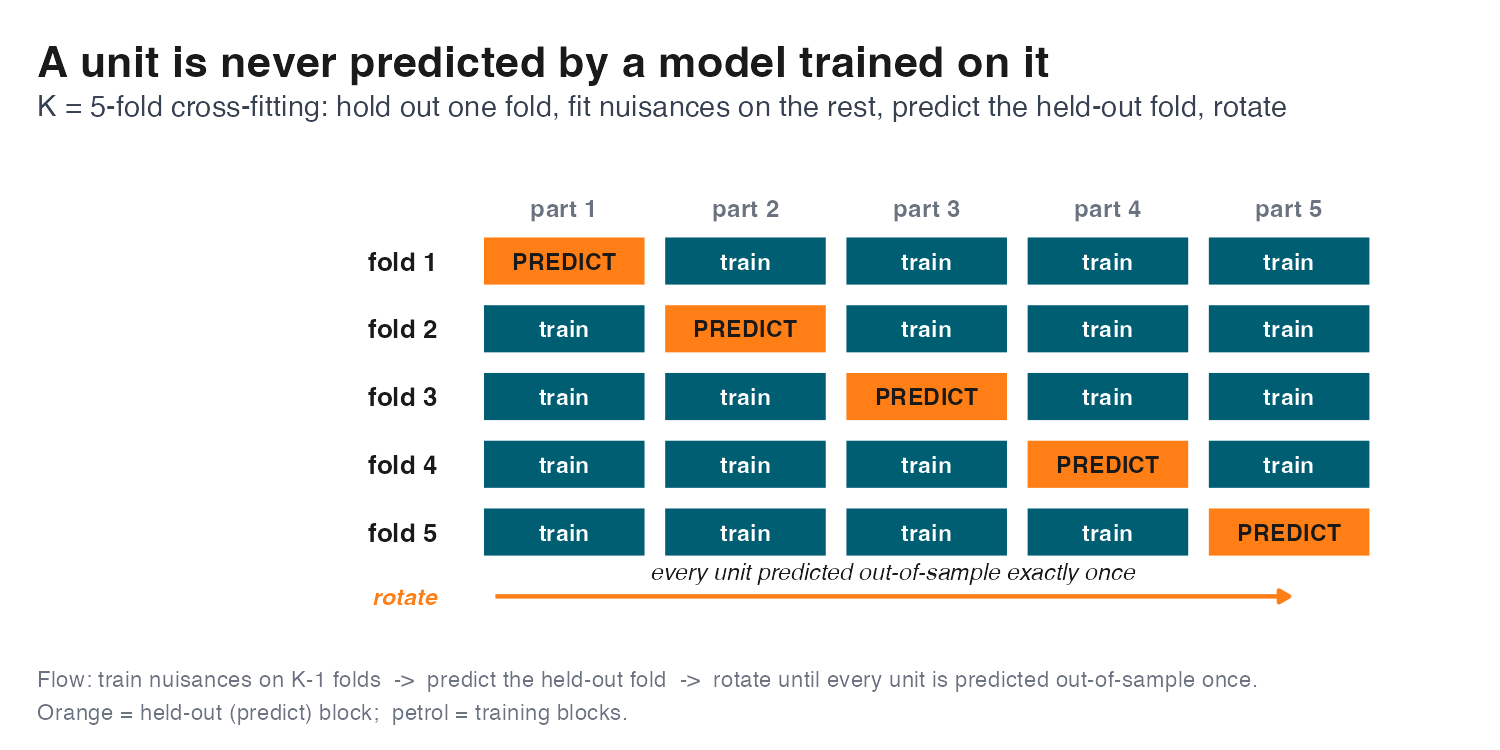
These out-of-fold predictions (Figure 12.4) are independent of each unit’s own noise, which decouples the nuisance-estimation error from the moment evaluation and makes the influence-function standard error honest. Five folds is the workhorse default (two suffices for very large \(n\); more folds means more training data per fold at the cost of compute). Because the fold split is random, a single split injects a small amount of noise into the estimate, so good practice repeats the whole cross-fitting procedure \(n_{\text{rep}}\) times and reports the median estimate with appropriately aggregated standard errors. On learner choice, there is no need to gamble on one algorithm — Ahrens et al. show you can stack several learners inside DML and let the data weight them (Ahrens et al. 2025). A caveat worth internalising: in LearnLoop, a forest with too small an mtry cannot see the baseline_score \(\times\) prior_courses interaction and the estimate biases upward. Orthogonality buys robustness to small nuisance error, not to a learner that fundamentally cannot fit the surface. And cross-fitting governs only how the nuisances are predicted (out-of-fold) — turning the resulting per-unit scores into \(\hat\tau\) is the separate averaging step (the four-step recipe, step 3).
12.3.3.3 The payoff: only orthogonality and cross-fitting work
The two ingredients are not redundant; each fixes a different failure, and you need both. A Monte-Carlo experiment makes this unmistakable. Standardize the estimates as \((\hat\tau - \tau)/\widehat{\text{SE}}\) over many simulated samples; if inference is valid, the histogram should track the standard normal.
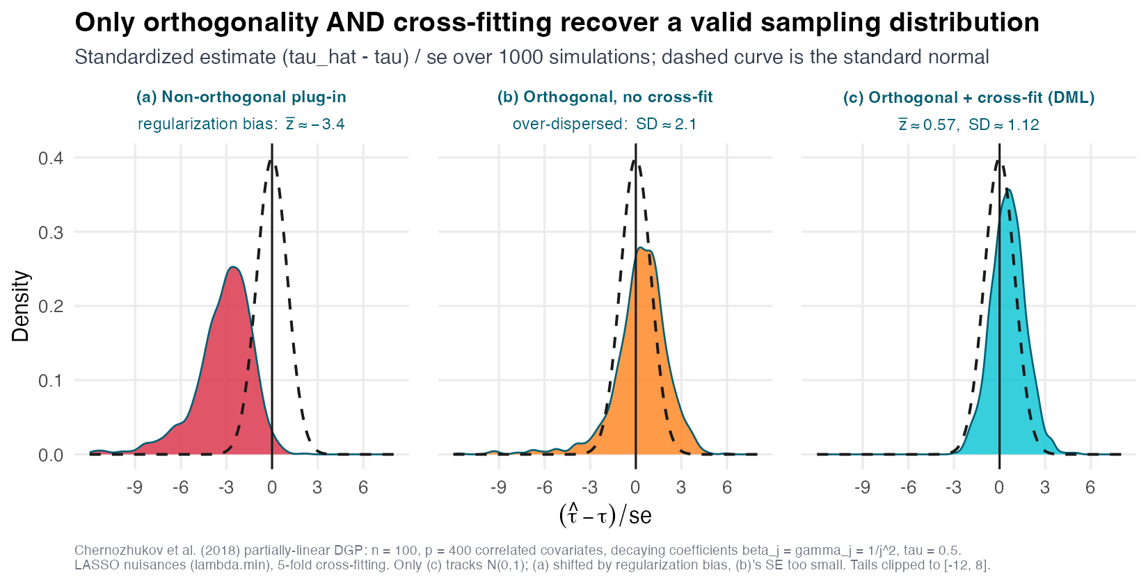
In Figure 12.5, panel (a) drops orthogonality: the distribution is shifted, betraying surviving regularization bias. Panel (b) keeps orthogonality but skips cross-fitting: the histogram is centred but too wide relative to the normal, so a nominal 95% interval covers the truth less than 95% of the time. Only panel (c), with both ingredients, hugs \(\mathcal{N}(0,1)\) — centred and correctly scaled. This figure is the empirical proof of the Chernozhukov et al. theorem in a single picture (Chernozhukov et al. 2018).
12.3.3.4 The recipe as a four-step checklist
Consolidating, the entire method is four steps, and it generalises: switch the score in step 1 and you switch the estimand, while steps 2–4 are identical across PLR, AIPW, and IV.
- Orthogonal score — choose a Neyman-orthogonal \(\psi\), linear in \(\tau\): \(\psi = \psi_a\,\tau + \psi_b\) (e.g. the Robinson moment \(\psi = (\tilde Y - \tau\,\tilde D)\,\tilde D\)).
- Cross-fitted nuisances — \(\hat\ell, \hat m\) from held-out folds; every unit predicted out-of-fold.
- Average & solve — set the empirical moment to zero, \(\mathbb{E}_n[\psi] = 0 \Rightarrow \hat\tau = -\,\mathbb{E}_n[\psi_b]/\mathbb{E}_n[\psi_a]\); for the Robinson score this is \(\sum_i \tilde Y_i\,\tilde D_i \,/\, \sum_i \tilde D_i^2\).
- Influence-function SE — with \(\phi_i = -\psi_i/\mathbb{E}_n[\psi_a]\), the standard error is \(\widehat{\text{SE}} = \sqrt{\widehat{\mathbb{E}}[\psi^2] \,/\, \widehat{\mathbb{E}}[\psi_a]^2 \,/\, n}\), the variance of the influence function rather than a naive plug-in (Chernozhukov et al. 2018).
Only the score (step 1) changes across models — steps 2–4 are identical. Throughout we write the effect \(\tau\); the DML papers and the DoubleML package write it \(\theta\) and report it as coef — the same object.
12.3.4 Two models, one recipe: PLR and AIPW
12.3.4.1 PLR in a few lines of DoubleML
The partially linear model is the recipe with the Robinson score. The DoubleML package makes it a three-liner with the same class names in both languages (Bach et al. 2024, 2022): declare the data, choose learners for the two nuisances (ml_l for \(\ell(\mathbf{X}) = \mathbb{E}[Y\mid\mathbf{X}]\) and ml_m for \(m(\mathbf{X}) = \mathbb{E}[D\mid\mathbf{X}]\)), set n_folds = 5, and fit; cross-fitting runs under the hood. On LearnLoop the estimate lands at \(\approx 5.0\) with a standard error near \(0.08\). The number arc is the whole pedagogical point: the naive comparison says \(+14.03\) (confounded), linear adjustment says \(+5.47\) (the interaction is missed and the CI excludes the truth), and DML lands at \(\approx 5.0\) (the interaction is caught). The coding lab builds this estimator by hand before reaching for the package.
12.3.4.2 The interactive model: when the effect is not a single number
PLR assumes one constant \(\tau\) — it forbids the treatment effect from depending on \(\mathbf{X}\). Relaxing that, the interactive regression model (IRM) fits the two potential-outcome surfaces and the propensity separately:
\[\mu_1(\mathbf{X}) = \mathbb{E}[Y\mid D=1, \mathbf{X}], \qquad \mu_0(\mathbf{X}) = \mathbb{E}[Y\mid D=0, \mathbf{X}], \qquad e(\mathbf{X}) = \mathbb{E}[D\mid\mathbf{X}].\]
The ATE is the average gap, \(\mathbb{E}[\mu_1(\mathbf{X}) - \mu_0(\mathbf{X})]\). But estimating it by the plug-in mean \(\frac{1}{n}\sum_i(\hat\mu_1(\mathbf{X}_i) - \hat\mu_0(\mathbf{X}_i))\) is not orthogonal — it inherits the regularization bias of Neyman orthogonality, because a shrunk \(\hat\mu_d\) leaves structure correlated with treatment assignment. We need an orthogonal score for the ATE, and that is AIPW.
12.3.4.3 AIPW = direct estimate + residual correction
The augmented inverse-propensity-weighted (AIPW) score, also called the doubly-robust score, repairs the plug-in with a propensity-weighted residual term (Robins, Rotnitzky, and Zhao 1994; Bang and Robins 2005):
\[\psi_i = \underbrace{\bigl[\hat\mu_1(\mathbf{X}_i) - \hat\mu_0(\mathbf{X}_i)\bigr]}_{\text{direct (outcome regression)}} \;+\; \underbrace{\frac{D_i\,(Y_i - \hat\mu_1(\mathbf{X}_i))}{\hat e(\mathbf{X}_i)} \;-\; \frac{(1-D_i)\,(Y_i - \hat\mu_0(\mathbf{X}_i))}{1-\hat e(\mathbf{X}_i)}}_{\text{bias correction (propensity-weighted residual)}}, \qquad \widehat{\text{ATE}} = \frac{1}{n}\sum_i \psi_i.\]
This is still the four-step engine — only the score changed. Writing \(\psi = \psi_i - \tau\) gives \(\psi_b = \psi_i\) and \(\psi_a = -1\). Step 2’s nuisances are now three, \((\mu_1, \mu_0, e)\) — PLR’s single \(m\) becomes two outcome arms plus the propensity — all cross-fitted. Because \(\psi_a = -1\), step 3 collapses to a plain average, \(\hat\tau = \mathbb{E}_n[\psi_i]\), and step 4’s influence-function SE reduces to \(\widehat{\text{SE}} = \sqrt{\widehat{\operatorname{Var}}(\psi_i)/n}\). Orthogonality and cross-fitting carry over verbatim.
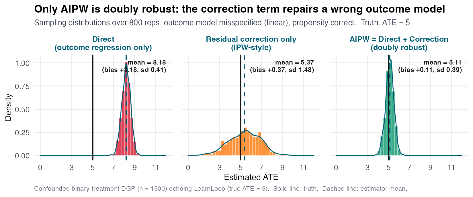
The direct part is the regression imputation of the per-unit gap; the correction part is the genius. Wherever the outcome model mispredicts, the propensity-weighted residual pushes back: when \(\hat\mu_d\) is correct the residuals are mean-zero and the correction adds only noise, but when \(\hat\mu_d\) is wrong the correction carries the estimate.
A Monte-Carlo experiment with the outcome model deliberately misspecified (fit linear when the truth is nonlinear) but the propensity correct makes the property visceral (Figure 12.6):
12.3.4.4 Overlap and positivity: check before you trust the weights
AIPW divides by \(\hat e(\mathbf{X})\) and \(1 - \hat e(\mathbf{X})\), so as propensities approach \(0\) or \(1\) the weights explode and the variance blows up. The diagnostic is simple and mandatory: plot the estimated propensity by treatment group and look for overlap (the positivity assumption that every covariate profile has a positive probability of either treatment). LearnLoop overlaps across most of \([0,1]\), but the forest’s raw scores still reach the tails — the worst inverse weight is several hundred — so the response to extreme propensities is not academic.
There are three such responses, and they are not the same operation:
| what it does to \(\hat e\) | estimand | when to use | |
|---|---|---|---|
| Trim | drops units with \(\hat e \notin [\alpha, 1-\alpha]\) | the overlap-ATE \(\neq\) ATE | genuine non-overlap |
| Clip | caps \(\hat e\) into \([\alpha, 1-\alpha]\), keeps every unit | full ATE, but capped units stay heavily weighted (widest SE) | a quick, blunt guard |
| Calibrate | rescales \(\hat e \to \tilde e\) so \(\mathbb{E}[D \mid \tilde e] = \tilde e\) | full ATE, with honest weights | ML over-confidence in the tails |
Only trimming changes the question — it re-defines the estimand to the ATE on the overlap subpopulation and discards data. Clip and calibrate both keep every unit and the full-population ATE, but clip patches the symptom (it bluntly caps the offending weights, so those units stay the most heavily weighted and the standard error is the widest) while calibrate fixes the cause: flexible ML propensities are routinely over-confident near \(0\) and \(1\), and a monotone recalibration (isotonic or Platt) pulls the scores back onto the \(45°\) reliability line, shrinking the inflated \(1/\hat e\) weights without dropping anyone. The practical default is therefore calibrate first, falling back to trimming only under genuine non-overlap (Ballinari and Bearth 2024; Crump et al. 2009). (Note that DoubleML’s trimming_rule = "truncate" is clipping, not dropping.) The coding lab makes all three concrete on LearnLoop and lines up their estimands and standard errors side by side.
12.3.5 When unconfoundedness fails: DML-IV
12.3.5.1 If a confounder is unobserved, bring back the instrument
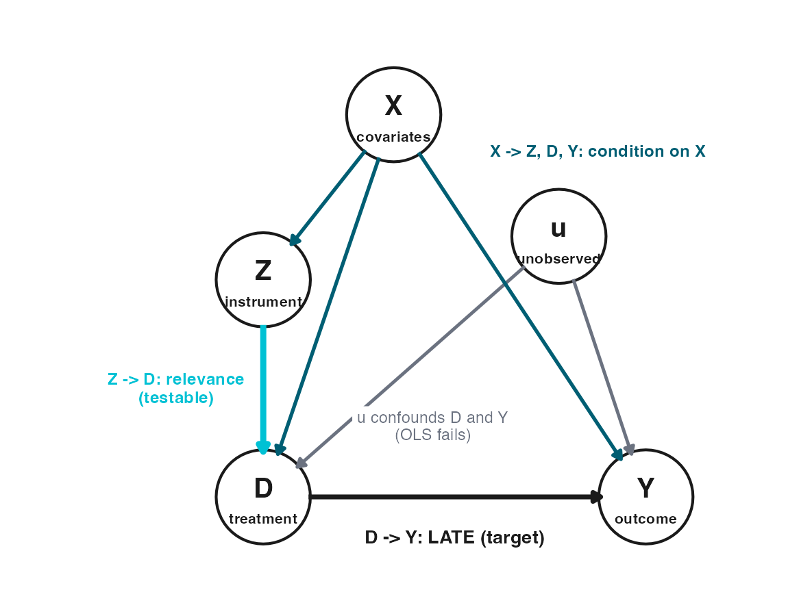
Everything so far has assumed unconfoundedness given \(\mathbf{X}\). When an unobserved \(u\) drives both \(D\) and \(Y\), no nuisance — however flexible — closes that backdoor, and DML’s machinery is powerless against it. The escape is exactly the S07 move: a valid instrument \(Z\) (here, a randomly-timed reminder) restores identification by harvesting a slice of variation in \(D\) that has no backdoor into \(Y\). The LearnLoop lesson-completion decision is the canonical case — latent student motivation \(u\) drives both whether a lesson is completed (\(D\)) and the subsequent exam score (\(Y\)) — so selection-on-observables fails and an instrument is required (Figure 12.7).
12.3.5.2 Partially linear IV (PLIV): instrument the residual
The first DML-IV estimator keeps PLR’s constant-\(\tau\) outcome equation but makes \(D\) endogenous; identification now rides on an instrument \(Z\) that is exogenous given \(\mathbf{X}\): \[Y = \tau\,D + g(\mathbf{X}) + \varepsilon, \quad \mathbb{E}[\varepsilon \mid Z, \mathbf{X}] = 0, \qquad Z = r(\mathbf{X}) + \nu, \quad \mathbb{E}[\nu \mid \mathbf{X}] = 0.\] There are now three nuisances — \(\ell = \mathbb{E}[Y\mid\mathbf{X}]\), \(m = \mathbb{E}[D\mid\mathbf{X}]\), and the instrument predictor \(r = \mathbb{E}[Z\mid\mathbf{X}]\) — giving residuals \(\tilde Y, \tilde D, \tilde Z\). The orthogonal score swaps the instrument residual \(\tilde Z\) in for \(\tilde D\) in the moment: \[\psi = (\tilde Y - \tau\,\tilde D)\,\tilde Z = \underbrace{(-\tilde D\tilde Z)}_{\psi_a}\,\tau + \underbrace{\tilde Y\tilde Z}_{\psi_b},\] so the closed-form root is the residualized Wald/2SLS estimand \(\hat\tau = \operatorname{Cov}(\tilde Y, \tilde Z)/\operatorname{Cov}(\tilde D, \tilde Z)\) and the influence function delivers the heteroskedasticity-robust IV standard error. It is PLR with exactly one change — \(\psi_a = -\tilde D\tilde Z\) in place of \(-\tilde D^2\), i.e. instrument the residual — and DoubleMLPLIV implements it (Robinson 1988). (A weak instrument, \(\operatorname{Cov}(\tilde D, \tilde Z) \approx 0\), blows up both the estimate and its SE — the DML echo of S07’s weak-IV problem.)
12.3.5.3 Interactive IV (IIVM): the LATE on compliers
When the treatment effect is not constant, the interactive IV model (IIVM) drops PLR’s single \(\tau\) and lets \(D\) enter the outcome surface arbitrarily, keeping the instrument exogenous given \(\mathbf{X}\). Its three nuisances are \(\mu(Z,\mathbf{X}) = \mathbb{E}[Y\mid Z,\mathbf{X}]\), \(p(Z,\mathbf{X}) = \mathbb{E}[D\mid Z,\mathbf{X}]\), and the instrument propensity \(r(\mathbf{X}) = \mathbb{E}[Z\mid\mathbf{X}]\). The orthogonal score is a ratio of two AIPW signals — \(\psi = \Gamma^Y - \tau\,\Gamma^D\), so \(\psi_b = \Gamma^Y\) and \(\psi_a = -\Gamma^D\) (AIPW had \(\psi_a = -1\)) — and solving gives the covariate-adjusted Wald ratio \(\hat\tau_{\text{LATE}} = \mathbb{E}_n[\Gamma^Y]/\mathbb{E}_n[\Gamma^D]\) (Frölich 2007), the intention-to-treat over the complier share. It targets the LATE, the average effect on compliers, just as 2SLS did in S07, and step 4 reads the influence-function SE off the same machinery. The crucial point of restraint: DML-IV neither weakens nor strengthens the identifying assumptions. Relevance, exclusion, and monotonicity are inherited verbatim from S07; DML contributes only the freedom to let the covariates enter the nuisances nonparametrically (Chernozhukov et al. 2018). On the encouragement data (where the true structural effect of completing is \(+6\) by construction), DoubleMLIIVM recovers a LATE \(\approx 6\) — the effect among the compliers the reminder actually moves — whereas a naive OLS of completing on exam score is biased upward by motivation (Knaus 2022). Here it is one more instance of the recipe with only the score changed.
12.3.6 How wrong could I be? Sensitivity and the bridge to S09
12.3.6.1 Unconfoundedness is an assumption, not a result
DML estimates the effect assuming \(\mathbf{X}\) is a sufficient adjustment set; it never proves it. If a relevant confounder is unmeasured, the ATE is still biased, and orthogonality will not save you — orthogonality concerns sensitivity to nuisance estimation error, not to identification failure. So we close the honesty loop exactly as S06 did: rather than test the untestable, we ask how strong an unobserved confounder would have to be to overturn the finding (Cinelli and Hazlett 2020).
12.3.6.2 OVB for ML: two strengths, their alignment, and a robustness value
The omitted-variable-bias framework generalises to the DML world (Chernozhukov et al. 2026). The bias from an omitted confounder \(U\) is the product of two errors, \(\text{bias} = \mathbb{E}\bigl[(g_0 - \hat g)(\alpha_0 - \hat\alpha)\bigr]\), where \(g = \mathbb{E}[Y\mid D,\mathbf{X}]\) is the outcome regression and \(\alpha\) is the score’s treatment-side object. The outcome side is always a regression, so \(cf_y\) — the partial \(R^2\) of \(U\) with the outcome — is always an ordinary partial \(R^2\). The treatment dial is score-dependent, though: for DML-PLR/PLIV (partialling-out) \(\alpha\) is the normalised residual \(\tilde D\), so \(cf_d\) is a plain partial \(R^2\) — exactly the S06 sensemakr quantity; for DML-AIPW/IRM/IIVM the estimand rides on inverse-propensity weights with no treatment coefficient, so \(\alpha = D/e - (1-D)/(1-e)\) is the Riesz representer and \(cf_d\) is the increase in its Riesz norm \(\mathbb{E}[\alpha^2]\) — a genuinely new quantity. This is the same “only the score changes” spine extended to sensitivity: the score sets \(\alpha\), and \(\alpha\) sets the treatment dial.
Cauchy–Schwarz turns the bias product into magnitudes times a correlation, exposing a third dial: \[|\text{bias}| = \underbrace{|\rho|}_{\text{alignment}} \cdot \underbrace{\sqrt{cf_y}}_{\text{outcome}} \cdot \underbrace{\sqrt{\tfrac{cf_d}{1 - cf_d}}}_{\text{treatment}} \cdot\, S,\] where \(\rho = \operatorname{Corr}(g_0 - \hat g,\ \alpha_0 - \hat\alpha)\) is the alignment of \(U\)’s two pulls and \(S\) is a scale fixed by the data. The alignment is decisive: \(\rho = 0\) gives zero bias even if \(U\) is arbitrarily strong, while \(\rho = \pm 1\) is the worst case. We report the worst case \(\rho = 1\), so the argument reduces to strength alone — and the robustness value (RV) is the common dial strength (at \(\rho = 1\)) that would drive the estimate to zero.
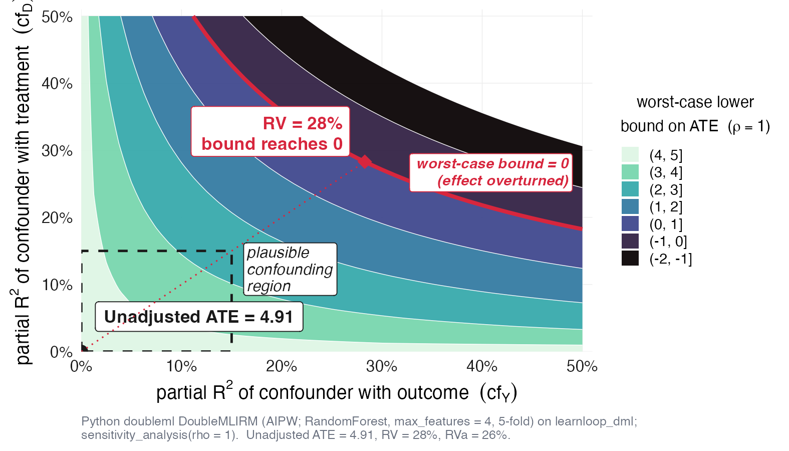
Reading the contour (Figure 12.8) like the S06 sensemakr plot: the highlighted contour marks where the worst-case lower bound on the ATE hits zero, and the robustness value is how far out one must travel to get there. Here — at the worst-case alignment \(\rho = 1\) — a confounder would have to explain about \(28\%\) of the residual variation in both the outcome and the treatment side to overturn the recommendation effect (the contour is the AIPW/IRM ATE case, so \(cf_d\) is the Riesz-norm dial; a PLR/PLIV effect would give the plain-sensemakr version). That is roughly twice the \(\approx 15\%\) the observed covariates themselves explain — a comfortable but not enormous margin, so the finding is robust with a \(\sim 2\times\) cushion rather than immune to any conceivable confounder. The lesson for practice: report an RV alongside every DML estimate, and pair it with a named industry workflow — Booking.com’s published sensitivity use case is a good template for “estimate, then stress-test, before acting” (Bach et al. 2025).
12.3.6.3 You do not have to hand-derive the correction
Every score in this session needed a bespoke correction term — the residual in PLR, the propensity-weighted residual in AIPW, the extra nuisance in IIVM. For a broad class of target functionals, that correction need not be derived by hand at all.
12.3.6.4 Recap and the bridge to S09
Four ideas carry the session. FWL with a machine: partial \(\mathbf{X}\) out of \(Y\) and \(D\) with any learner, then read the slope. Two ingredients: orthogonality kills regularization bias, cross-fitting kills overfitting bias, and together they restore the \(\sqrt{n}\), asymptotically normal confidence interval. One score per estimand: PLR for a constant effect, AIPW/IRM for the doubly-robust ATE, IIVM for the LATE — steps 2–4 never change. And the guardrail: DML solves estimation, not identification, so always stress-test unconfoundedness.
The bridge to next week is the per-unit score. S08 averages \(\psi_i\) to the ATE; S09 stops averaging and starts projecting \(\psi_i\) on \(\mathbf{X}\) to recover heterogeneous effects \(\tau(x)\) — the doubly-robust learner, meta-learners, and causal forests are all variations on that single move (Wager and Athey 2018). The same orthogonal-score logic also powers difference-in-differences in Part V (Chang 2020). DML is a powerful estimator, never a substitute for a credible identification argument.
12.4 Coding Lab
The lab works the LearnLoop recommendation problem end to end on a synthetic dataset where the truth is known (the true ATE of the recommendation on exam score \(= +5.0\) points). The arc is by hand, then by package: first build each estimator from cross-fitting primitives so the machinery is transparent, then confirm with DoubleML. Each exercise gives a Scaffold with # ___ YOUR CODE placeholders in both R and Python; attempt it, then expand Show solution to compare. The primary dataset is materials/data/learnloop_dml.csv; the optional IV exercise uses materials/data/learnloop_iv.csv. One detail matters throughout: pass mtry = 4 (R ranger) / max_features = 4 (scikit-learn) — the default considers too few features per split to see the baseline_score × prior_courses interaction, and the estimate drifts upward.
Download the datasets: learnloop_dml.csv · learnloop_iv.csv
12.4.1 Exercise 1 — Partialling-out by hand (~25 min)
Build the partially linear DML estimator from scratch: residualize \(Y\) and \(D\) against \(\mathbf{X}\) with a cross-fitted random forest, then read the residual-on-residual slope. Compare it to the naive contrast and to linear adjustment — the gap between linear adjustment and DML is the value the machine adds.
12.4.1.1 Scaffold
import numpy as np, pandas as pd
from sklearn.ensemble import RandomForestRegressor
from sklearn.model_selection import KFold
import statsmodels.api as sm

CAT = ["gender", "region", "device", "track"]
np.random.seed(42)
df = pd.read_csv("../../materials/data/learnloop_dml.csv")
df = pd.get_dummies(df, columns=CAT, drop_first=True)          # NB: yields bool cols
y = df["exam_score"].to_numpy(dtype=float)
d = df["recommended"].to_numpy().astype(float)
X = df.drop(columns=["exam_score", "recommended"]).to_numpy(dtype=float)
n = len(y)

# (a) Contrasts: naive Y~D, then linear-controls OLS Y~D+X
# ___ YOUR CODE: sm.OLS(y, sm.add_constant(d)).fit()
# ___ YOUR CODE: sm.OLS(y, sm.add_constant(np.column_stack([d, X]))).fit()

# (b) 5-fold cross-fit l_hat=E[Y|X], m_hat=E[D|X] with RandomForest (max_features=4!)
kf = KFold(n_splits=5, shuffle=True, random_state=42)
l_hat, m_hat = np.zeros(n), np.zeros(n)
for tr, te in kf.split(X):
    # ___ YOUR CODE: fit RandomForestRegressor(n_estimators=500, max_features=4, random_state=42)
    # ___ YOUR CODE: l_hat[te] = ...predict(X[te]) ; same for m_hat on d
    pass

# (c) residualize, (d) solve the moment + influence-function SE — does the CI cover 5.0?
# ___ YOUR CODE
TipShow solution
suppressPackageStartupMessages({
  library(readr); library(dplyr); library(data.table)
  library(ranger); library(fixest)
})

covars <- c("age","gender","region","prior_courses",
            "baseline_score","device","track")

set.seed(42)
df <- read_csv(here::here("materials/data/learnloop_dml.csv"), show_col_types = FALSE) |>
  mutate(across(c(gender, region, device, track), as.factor))

# --- contrasts: naive and linear-controls OLS ---
naive <- feols(exam_score ~ recommended, data = df)
lin   <- feols(exam_score ~ recommended + age + gender + region +
                 prior_courses + baseline_score + device + track,
               data = df)
cat(sprintf("Naive  Y~D            : %.4f\n", coef(naive)["recommended"]))
Naive Y~D : 14.0324cat(sprintf("Linear-controls OLS : %.4f\n", coef(lin)["recommended"]))Linear-controls OLS : 5.4701# --- 5-fold cross-fitting ---
n <- nrow(df); n_folds <- 5
folds <- sample(rep(1:n_folds, length.out = n))
Y <- df$exam_score; D <- df$recommended
Xdf <- df[, covars]
l_hat <- numeric(n) # E[Y|X]
m_hat <- numeric(n) # E[D|X]
for (k in 1:n_folds) {
tr <- folds != k; te <- folds == k
fitY <- ranger(x = Xdf[tr, ], y = Y[tr], num.trees = 500, mtry = 4)
fitD <- ranger(x = Xdf[tr, ], y = D[tr], num.trees = 500, mtry = 4)
l_hat[te] <- predict(fitY, Xdf[te, ])$predictions
m_hat[te] <- predict(fitD, Xdf[te, ])$predictions
}
res_y <- Y - l_hat
res_d <- D - m_hat
tau_plr <- sum(res_y * res_d) / sum(res_d^2)
# influence-function SE
psi_a <- -res_d^2
psi_b <- res_y * res_d
psi <- psi_b + psi_a * tau_plr
J <- mean(psi_a)
se_plr <- sqrt(mean(psi^2) / J^2) / sqrt(n)
ci_plr <- tau_plr + c(-1, 1) * 1.96 * se_plr
cat(sprintf("PLR tau (by hand) : %.4f (SE %.4f)\n", tau_plr, se_plr))PLR tau (by hand) : 5.0698 (SE 0.0759)cat(sprintf("PLR 95%% CI : [%.4f, %.4f]\n", ci_plr[1], ci_plr[2]))PLR 95% CI : [4.9210, 5.2186]import numpy as np
import pandas as pd
from sklearn.ensemble import RandomForestRegressor
from sklearn.model_selection import KFold
import statsmodels.api as sm
CAT = ["gender", "region", "device", "track"]
np.random.seed(42)
df = pd.read_csv("../../materials/data/learnloop_dml.csv")
df = pd.get_dummies(df, columns=CAT, drop_first=True)
y = df["exam_score"].to_numpy(dtype=float)
d = df["recommended"].to_numpy().astype(float)
# get_dummies yields bool columns -> cast to float for sklearn/statsmodels
X = df.drop(columns=["exam_score", "recommended"]).to_numpy(dtype=float)
n = len(y)
naive = sm.OLS(y, sm.add_constant(d)).fit()
print(f"Naive Y~D coef on D: {naive.params[1]:.4f}")Naive Y~D coef on D: 14.0324Xlin = sm.add_constant(np.column_stack([d, X]))
ols = sm.OLS(y, Xlin).fit()
print(f"Linear-controls OLS on D: {ols.params[1]:.4f}")Linear-controls OLS on D: 5.4701kf = KFold(n_splits=5, shuffle=True, random_state=42)
l_hat = np.zeros(n); m_hat = np.zeros(n)
for tr, te in kf.split(X):
rf_l = RandomForestRegressor(n_estimators=500, max_features=4, random_state=42)
rf_m = RandomForestRegressor(n_estimators=500, max_features=4, random_state=42)
l_hat[te] = rf_l.fit(X[tr], y[tr]).predict(X[te])
m_hat[te] = rf_m.fit(X[tr], d[tr]).predict(X[te])
res_y = y - l_hat
res_d = d - m_hat
tau = np.sum(res_y * res_d) / np.sum(res_d ** 2)
# influence-function SE (same psi_a / psi_b convention as the R tab and the slides)
psi_a = -res_d ** 2 # coefficient on tau
psi_b = res_y * res_d # constant part
psi = psi_b + psi_a * tau # full score at tau
J = np.mean(psi_a)
se = np.sqrt(np.mean(psi ** 2) / J ** 2 / n)
ci = (tau - 1.96 * se, tau + 1.96 * se)
print(f"PLR by-hand tau: {tau:.4f}")PLR by-hand tau: 5.0684print(f"PLR by-hand SE: {se:.4f}")PLR by-hand SE: 0.0747print(f"PLR 95% CI: [{ci[0]:.4f}, {ci[1]:.4f}]")PLR 95% CI: [4.9220, 5.2148]print(f"CI covers 5.0: {ci[0] <= 5.0 <= ci[1]}")CI covers 5.0: TrueThe naive contrast (≈ 14.03) is grossly confounded; linear adjustment (≈ 5.47) is close but its CI excludes 5.0 because the linear spec omits the baseline-score × prior-courses interaction; the cross-fitted forest residualization recovers ≈ 5.0 with a CI that covers the truth. R and Python use independent random-number streams, so the third decimal differs — the conclusion does not.
12.4.2 Exercise 2 — AIPW by hand, and the overlap check (~25 min)
Code the doubly-robust score directly. Cross-fit the two outcome surfaces \(\mu_1, \mu_0\) and the propensity \(e\), assemble the per-unit AIPW score, and average. First inspect the propensity histogram — AIPW divides by \(\hat e\) and \(1-\hat e\), so overlap is a precondition, not an afterthought.
12.4.2.1 Scaffold
# Reuses df, covars, n, n_folds, Y, D, Xdf from Exercise 1
set.seed(42)
folds2 <- sample(rep(1:n_folds, length.out = n))
mu1 <- mu0 <- e_hat <- numeric(n)
for (k in 1:n_folds) {
  tr <- folds2 != k; te <- folds2 == k
  # ___ YOUR CODE: fit mu1 on treated-in-train, mu0 on control-in-train, e on all-train
  # ___ YOUR CODE: predict mu1[te], mu0[te], e_hat[te]   (ranger, mtry = 4)
}
# ___ YOUR CODE: clip e_hat to [0.01, 0.99]; inspect quantiles (overlap)
# ___ YOUR CODE: psi <- (mu1 - mu0) + D*(Y - mu1)/e_hat - (1 - D)*(Y - mu0)/(1 - e_hat)
# ___ YOUR CODE: ATE = mean(psi); SE = sd(psi)/sqrt(n); 95% CI
# Reload as in Ex1 (df, y, d, X, n). Then cross-fit mu1, mu0, e_hat.
from sklearn.ensemble import RandomForestRegressor, RandomForestClassifier
mu1 = np.zeros(n); mu0 = np.zeros(n); e_hat = np.zeros(n)
for tr, te in kf.split(X):
tr1 = tr[d[tr] == 1]; tr0 = tr[d[tr] == 0]
# ___ YOUR CODE: fit RF on (X[tr1], y[tr1]) -> mu1[te]; (X[tr0], y[tr0]) -> mu0[te]
# ___ YOUR CODE: fit RandomForestClassifier on (X[tr], d[tr]) -> e_hat[te] (predict_proba[:,1])
pass
# ___ YOUR CODE: quantiles of e_hat (overlap); clip to [0.01, 0.99]
# ___ YOUR CODE: psi = (mu1 - mu0) + d*(y - mu1)/e_hat - (1 - d)*(y - mu0)/(1 - e_hat)
# ___ YOUR CODE: ATE = psi.mean(); SE = psi.std(ddof=1)/sqrt(n)
TipShow solution
# Reuses df, covars, n, n_folds, Y, D, Xdf from Exercise 1
set.seed(42)
folds2 <- sample(rep(1:n_folds, length.out = n))
mu1 <- numeric(n); mu0 <- numeric(n); e_hat <- numeric(n)
for (k in 1:n_folds) {
  tr <- folds2 != k; te <- folds2 == k
  tr1 <- tr & (D == 1); tr0 <- tr & (D == 0)
  fit1 <- ranger(x = Xdf[tr1, ], y = Y[tr1], num.trees = 500, mtry = 4)
  fit0 <- ranger(x = Xdf[tr0, ], y = Y[tr0], num.trees = 500, mtry = 4)
  fitP <- ranger(x = Xdf[tr, ],  y = D[tr],  num.trees = 500, mtry = 4)
  mu1[te]   <- predict(fit1, Xdf[te, ])$predictions
  mu0[te]   <- predict(fit0, Xdf[te, ])$predictions
  e_hat[te] <- predict(fitP, Xdf[te, ])$predictions
}
# trim e for overlap / numerical stability
e_raw <- e_hat                                  # keep the raw scores for the demo below
e_hat <- pmin(pmax(e_hat, 0.01), 0.99)
psi_aipw <- (mu1 - mu0) + D * (Y - mu1) / e_hat - (1 - D) * (Y - mu0) / (1 - e_hat)
ate_aipw <- mean(psi_aipw)
se_aipw  <- sd(psi_aipw) / sqrt(n)
ci_aipw  <- ate_aipw + c(-1, 1) * 1.96 * se_aipw
cat("Overlap: quantiles of e_hat (propensity):\n")
Overlap: quantiles of e_hat (propensity):print(round(quantile(e_hat, c(0, .01, .05, .25, .5, .75, .95, .99, 1)), 4)) 0% 1% 5% 25% 50% 75% 95% 99% 100%
0.0100 0.0259 0.0713 0.2584 0.4251 0.6313 0.8879 0.9727 0.9900 cat(sprintf("AIPW ATE (by hand) : %.4f (SE %.4f)\n", ate_aipw, se_aipw))AIPW ATE (by hand) : 5.0511 (SE 0.1417)cat(sprintf("AIPW 95%% CI : [%.4f, %.4f]\n", ci_aipw[1], ci_aipw[2]))AIPW 95% CI : [4.7735, 5.3288]from sklearn.ensemble import RandomForestRegressor, RandomForestClassifier
np.random.seed(42)
mu1 = np.zeros(n); mu0 = np.zeros(n); e_hat = np.zeros(n)
for tr, te in kf.split(X):
tr1 = tr[d[tr] == 1]
tr0 = tr[d[tr] == 0]
rf1 = RandomForestRegressor(n_estimators=500, max_features=4, random_state=42)
rf0 = RandomForestRegressor(n_estimators=500, max_features=4, random_state=42)
rfe = RandomForestClassifier(n_estimators=500, max_features=4, random_state=42)
mu1[te] = rf1.fit(X[tr1], y[tr1]).predict(X[te])
mu0[te] = rf0.fit(X[tr0], y[tr0]).predict(X[te])
e_hat[te] = rfe.fit(X[tr], d[tr]).predict_proba(X[te])[:, 1]
qs = np.quantile(e_hat, [0, .01, .05, .25, .5, .75, .95, .99, 1])
print("Overlap (e_hat quantiles):")Overlap (e_hat quantiles):for q, v in zip([0, 1, 5, 25, 50, 75, 95, 99, 100], qs):
print(f" {q:>3}%: {v:.4f}") 0%: 0.0020
1%: 0.0260
5%: 0.0680
25%: 0.2380
50%: 0.4200
75%: 0.6460
95%: 0.9000
99%: 0.9700
100%: 0.9980e_raw = e_hat.copy() # keep the raw scores for the demo below
e_hat = np.clip(e_hat, 0.01, 0.99)
psi = (mu1 - mu0) + d * (y - mu1) / e_hat - (1 - d) * (y - mu0) / (1 - e_hat)
ate = psi.mean()
se = psi.std(ddof=1) / np.sqrt(n)
ci = (ate - 1.96 * se, ate + 1.96 * se)
print(f"AIPW by-hand ATE: {ate:.4f}")AIPW by-hand ATE: 4.9524print(f"AIPW by-hand SE: {se:.4f}")AIPW by-hand SE: 0.1816print(f"AIPW 95% CI: [{ci[0]:.4f}, {ci[1]:.4f}]")AIPW 95% CI: [4.5965, 5.3083]The propensities cover most of \((0,1)\), so overlap holds across the bulk and the by-hand doubly-robust ATE recovers ≈ 5.0. But the forest’s raw scores do reach the tails — the worst inverse weight is several hundred — which is exactly where the choice between trimming, clipping, and calibrating bites. The next block makes all three concrete.
12.4.2.2 Overlap fix in practice: trim vs. clip vs. calibrate
Reusing the cross-fitted nuisances from Exercise 2 (mu1, mu0, and the raw propensity e_raw), put the three responses to extreme propensities side by side on the same scores. Fill in the three e vectors below, then decide which one changes the estimand and which only re-weight.
# Reuses mu1, mu0, e_raw, Y, D, n, folds2, n_folds from Exercise 2
aipw_ate <- function(mu1, mu0, Y, D, e) {
  psi <- (mu1 - mu0) + D * (Y - mu1) / e - (1 - D) * (Y - mu0) / (1 - e)
  c(ate = mean(psi), se = sd(psi) / sqrt(length(psi)))
}

# (1) TRIM — drop units with e_raw outside [0.05, 0.95]; the estimand becomes the overlap-ATE
# ___ YOUR CODE: keep <- e_raw >= 0.05 & e_raw <= 0.95
# ___ YOUR CODE: a_trim <- aipw_ate(mu1[keep], mu0[keep], Y[keep], D[keep], e_raw[keep])

# (2) CLIP — keep all units, bluntly cap e_raw into [0.01, 0.99]
# ___ YOUR CODE: e_clip <- pmin(pmax(e_raw, 0.01), 0.99); a_clip <- aipw_ate(mu1, mu0, Y, D, e_clip)

# (3) CALIBRATE — cross-fitted isotonic map e_raw -> realised D, fold by fold
e_cal <- numeric(n)
for (k in 1:n_folds) {
  tr <- folds2 != k; te <- folds2 == k
  # ___ YOUR CODE: e_cal[te] <- approxfun(sort(e_raw[tr]), isoreg(e_raw[tr], D[tr])$yf, rule = 2)(e_raw[te])
}
# ___ YOUR CODE: a_cal <- aipw_ate(mu1, mu0, Y, D, pmin(pmax(e_cal, 0.01), 0.99))
# Compare a_trim / a_clip / a_cal.
from sklearn.isotonic import IsotonicRegression
# Reuses mu1, mu0, e_raw, y, d, n, X, kf from Exercises 1-2
def aipw_ate(mu1, mu0, y, d, e):
psi = (mu1 - mu0) + d * (y - mu1) / e - (1 - d) * (y - mu0) / (1 - e)
return psi.mean(), psi.std(ddof=1) / np.sqrt(len(psi))
# (1) TRIM -> overlap-ATE: keep e_raw in [0.05, 0.95]
# ___ YOUR CODE: keep = (e_raw >= 0.05) & (e_raw <= 0.95)
# ___ YOUR CODE: a_trim = aipw_ate(mu1[keep], mu0[keep], y[keep], d[keep], e_raw[keep])
# (2) CLIP -> full ATE, blunt cap into [0.01, 0.99]
# ___ YOUR CODE: a_clip = aipw_ate(mu1, mu0, y, d, np.clip(e_raw, 0.01, 0.99))
# (3) CALIBRATE -> full ATE, cross-fitted isotonic, fold by fold
e_cal = np.zeros(n)
for tr, te in kf.split(X):
# ___ YOUR CODE: iso = IsotonicRegression(out_of_bounds="clip", y_min=0, y_max=1).fit(e_raw[tr], d[tr])
# ___ YOUR CODE: e_cal[te] = iso.transform(e_raw[te])
pass
# ___ YOUR CODE: a_cal = aipw_ate(mu1, mu0, y, d, np.clip(e_cal, 0.01, 0.99))
# Compare a_trim / a_clip / a_cal.
TipShow solution
# Reuses mu1, mu0, e_raw, Y, D, n, folds2, n_folds from Exercise 2
aipw_ate <- function(mu1, mu0, Y, D, e) {
  psi <- (mu1 - mu0) + D * (Y - mu1) / e - (1 - D) * (Y - mu0) / (1 - e)
  c(ate = mean(psi), se = sd(psi) / sqrt(length(psi)))
}

# (1) TRIM  — drop tail units; the estimand becomes the overlap-ATE
keep   <- e_raw >= 0.05 & e_raw <= 0.95
a_trim <- aipw_ate(mu1[keep], mu0[keep], Y[keep], D[keep], e_raw[keep])

# (2) CLIP  — keep all units, bluntly cap e in [0.01, 0.99]
e_clip <- pmin(pmax(e_raw, 0.01), 0.99)
a_clip <- aipw_ate(mu1, mu0, Y, D, e_clip)

# (3) CALIBRATE — keep all units; cross-fitted isotonic map  e_raw -> realised D
e_cal <- numeric(n)
for (k in 1:n_folds) {
  tr <- folds2 != k; te <- folds2 == k
  e_cal[te] <- approxfun(sort(e_raw[tr]), isoreg(e_raw[tr], D[tr])$yf, rule = 2)(e_raw[te])
}
e_cal <- pmin(pmax(e_cal, 0.01), 0.99)
a_cal <- aipw_ate(mu1, mu0, Y, D, e_cal)

cat(sprintf("Raw propensity in [%.3f, %.3f]  ->  worst IPW weight 1/min(e) = %.0f\n\n",
            min(e_raw), max(e_raw), 1 / min(e_raw)))
Raw propensity in [0.002, 1.000] -> worst IPW weight 1/min(e) = 500cat(sprintf("%-24s %-12s %6s %8s %7s\n", "method", "estimand", "n", "ATE", "SE"))method estimand n ATE SEcat(sprintf("%-24s %-12s %6d %8.3f %7.3f\n", "Trim (drop tails)", "overlap-ATE", sum(keep), a_trim["ate"], a_trim["se"]))Trim (drop tails) overlap-ATE 9519 5.150 0.101cat(sprintf("%-24s %-12s %6d %8.3f %7.3f\n", "Clip (cap .01/.99)", "full ATE", n, a_clip["ate"], a_clip["se"]))Clip (cap .01/.99) full ATE 10000 5.051 0.142cat(sprintf("%-24s %-12s %6d %8.3f %7.3f\n", "Calibrate (isotonic)", "full ATE", n, a_cal["ate"], a_cal["se"]))Calibrate (isotonic) full ATE 10000 5.241 0.115# reliability diagram: raw scores sit off the 45-degree line; calibrated ones hug it
br <- seq(0, 1, 0.1); b <- cut(e_raw, br, include.lowest = TRUE); bc <- cut(e_cal, br, include.lowest = TRUE)
plot(tapply(e_raw, b, mean), tapply(D, b, mean), type = "b", pch = 19, col = "#D7263D",
xlim = 0:1, ylim = 0:1, xlab = "mean predicted propensity", ylab = "actual treatment rate",
main = "Reliability: raw (red) vs calibrated (blue)")
lines(tapply(e_cal, bc, mean), tapply(D, bc, mean), type = "b", pch = 17, col = "#00C1D4")
abline(0, 1, lty = 2, col = "grey50")
from sklearn.isotonic import IsotonicRegression
from sklearn.calibration import calibration_curve
import matplotlib.pyplot as plt
# Reuses mu1, mu0, e_raw, y, d, n, X, kf from Exercises 1-2
def aipw_ate(mu1, mu0, y, d, e):
    psi = (mu1 - mu0) + d * (y - mu1) / e - (1 - d) * (y - mu0) / (1 - e)
    return psi.mean(), psi.std(ddof=1) / np.sqrt(len(psi))

# (1) TRIM -> overlap-ATE
keep = (e_raw >= 0.05) & (e_raw <= 0.95)
at = aipw_ate(mu1[keep], mu0[keep], y[keep], d[keep], e_raw[keep])

# (2) CLIP -> full ATE, blunt cap
ac = aipw_ate(mu1, mu0, y, d, np.clip(e_raw, 0.01, 0.99))

# (3) CALIBRATE -> full ATE, cross-fitted isotonic
e_cal = np.zeros(n)
for tr, te in kf.split(X):
    iso = IsotonicRegression(out_of_bounds="clip", y_min=0, y_max=1).fit(e_raw[tr], d[tr])
    e_cal[te] = iso.transform(e_raw[te])
e_cal = np.clip(e_cal, 0.01, 0.99)
aa = aipw_ate(mu1, mu0, y, d, e_cal)

print(f"Raw propensity in [{e_raw.min():.3f}, {e_raw.max():.3f}]  ->  worst IPW weight {1/e_raw.min():.0f}\n")
Raw propensity in [0.002, 0.998] -> worst IPW weight 500print(f"{'method':24}{'estimand':12}{'n':>6}{'ATE':>9}{'SE':>8}")method estimand n ATE SEprint(f"{'Trim (drop tails)':24}{'overlap-ATE':12}{keep.sum():>6}{at[0]:>9.3f}{at[1]:>8.3f}")Trim (drop tails) overlap-ATE 9461 5.107 0.111print(f"{'Clip (cap .01/.99)':24}{'full ATE':12}{n:>6}{ac[0]:>9.3f}{ac[1]:>8.3f}")Clip (cap .01/.99) full ATE 10000 4.952 0.182print(f"{'Calibrate (isotonic)':24}{'full ATE':12}{n:>6}{aa[0]:>9.3f}{aa[1]:>8.3f}")Calibrate (isotonic) full ATE 10000 5.378 0.138fr, mp = calibration_curve(d, e_raw, n_bins=10, strategy="uniform")
frc, mpc = calibration_curve(d, e_cal, n_bins=10, strategy="uniform")
plt.figure(figsize=(6, 4)); plt.plot([0, 1], [0, 1], "--", color="grey")
plt.plot(mp, fr, "o-", color="#D7263D", label="raw")
plt.plot(mpc, frc, "^-", color="#00C1D4", label="calibrated")
plt.xlabel("mean predicted propensity"); plt.ylabel("actual treatment rate")
plt.title("Reliability: raw vs calibrated"); plt.legend(); plt.tight_layout(); plt.show()
All three land near the true ATE of \(5.0\), but they are not the same operation. Trimming drops the tail units (here \(\hat e\notin[0.05,0.95]\), a wider band than clip’s cap), so it estimates the overlap-ATE on a smaller population — a different estimand, not the full-population ATE. Clipping keeps every unit and the full estimand but caps the tail propensities bluntly, so those units still carry the heaviest weights and its SE is the widest. Calibration rescales \(\hat e\) to honest values — the reliability curve moves from off-diagonal (the forest is over-confident: it predicts \(\approx 0.95\) in the top bin where only \(\approx 0.89\) are truly treated) onto the \(45°\) line — keeping every unit and the full ATE while shrinking the variance relative to clipping. On LearnLoop, where overlap is only mild, the three point estimates stay close to \(5.0\) (calibration runs slightly high here); the principled reason to prefer calibration is that it fixes the cause (over-confident scores) rather than the symptom (huge weights), without changing the question — and the gap widens as overlap degrades. (Note: DoubleML’s trimming_rule = "truncate" is clipping, not dropping.)
12.4.3 Exercise 3 — Verify with DoubleML, then sensitivity-test (~25 min)
Reproduce the by-hand estimates with the production package — DoubleMLPLR and DoubleMLIRM should agree with Exercises 1–2 — then run a sensitivity analysis: how strong would an unobserved confounder have to be to overturn the result? Read the answer off DoubleML’s native sensitivity_summary (the robustness value) and sensitivity_plot (a contour of the worst-case bound). This is built into Python DoubleML; the R package has no equivalent, so the sensitivity step lives in the Python tab.
12.4.3.1 Scaffold
library(data.table); library(DoubleML); library(mlr3); library(mlr3learners)
lgr::get_logger("mlr3")$set_threshold("warn")
dt <- as.data.table(df)                 # DoubleML needs a data.table
dml_data <- DoubleMLData$new(dt, y_col = "exam_score",
                             d_cols = "recommended", x_cols = covars)
# ___ YOUR CODE: DoubleMLPLR$new(dml_data, ml_l = lrn("regr.ranger", mtry = 4), ml_m = ..., n_folds = 5)$fit()
# ___ YOUR CODE: DoubleMLIRM$new(dml_data, ml_g = regr.ranger, ml_m = classif.ranger(prob), score = "ATE")$fit()
#                NB: R DoubleML has no sensitivity_analysis() — the sensitivity step is Python-only (see the Python tab)
import doubleml as dml
from sklearn.ensemble import RandomForestRegressor, RandomForestClassifier
x_cols = [c for c in df.columns if c not in ["exam_score", "recommended"]]
dml_data = dml.DoubleMLData(df, y_col="exam_score",
d_cols="recommended", x_cols=x_cols)
# ___ YOUR CODE: dml.DoubleMLPLR(dml_data, ml_l=RF(max_features=4), ml_m=RF(...), n_folds=5).fit()
# ___ YOUR CODE: dml.DoubleMLIRM(dml_data, ml_g=RF, ml_m=RFClassifier, score="ATE").fit()
# ___ YOUR CODE: irm.sensitivity_analysis(cf_y=0.03, cf_d=0.03); print(irm.sensitivity_summary) # bounds + RV/RVa
# ___ YOUR CODE: irm.sensitivity_plot(grid_bounds=(0.5, 0.5)).show() # native contour
TipShow solution
suppressPackageStartupMessages({
  library(data.table); library(DoubleML); library(mlr3); library(mlr3learners)
})
lgr::get_logger("mlr3")$set_threshold("warn")

dt <- as.data.table(df)
dml_data <- DoubleMLData$new(dt, y_col = "exam_score",
                             d_cols = "recommended", x_cols = covars)

# --- PLR ---
set.seed(42)
ml_l <- lrn("regr.ranger", num.trees = 500, mtry = 4, seed = 42)
ml_m <- lrn("regr.ranger", num.trees = 500, mtry = 4, seed = 42)
dml_plr <- DoubleMLPLR$new(dml_data, ml_l = ml_l, ml_m = ml_m, n_folds = 5)
dml_plr$fit()
cat(sprintf("DoubleML PLR coef     : %.4f  (SE %.4f)\n", dml_plr$coef, dml_plr$se))
DoubleML PLR coef : 5.0614 (SE 0.0759)# --- IRM (ATE) ---
set.seed(42)
ml_g <- lrn("regr.ranger", num.trees = 500, mtry = 4, seed = 42)
ml_mc <- lrn("classif.ranger", num.trees = 500, mtry = 4,
predict_type = "prob", seed = 42)
dml_irm <- DoubleMLIRM$new(dml_data, ml_g = ml_g, ml_m = ml_mc,
n_folds = 5, score = "ATE")
dml_irm$fit(store_predictions = TRUE) # NB: store_predictions is a fit() argument
cat(sprintf("DoubleML IRM coef : %.4f (SE %.4f)\n", dml_irm$coef, dml_irm$se))DoubleML IRM coef : 5.0198 (SE 0.1476)# --- Sensitivity: not available in R DoubleML ---
# R DoubleML has no sensitivity_analysis(). The only R option is the GitHub-only
# package dml.sensemakr (Chernozhukov et al. 2026), but it refits the DML with its
# own engine, so it reports a different point estimate and robustness value than the
# DoubleMLIRM above. To keep one estimate per estimand, we run the sensitivity
# analysis natively in Python (see the Python tab) -- the robustness value is ~28%.import doubleml as dml
from sklearn.ensemble import RandomForestRegressor, RandomForestClassifier
np.random.seed(42)
x_cols = [c for c in df.columns if c not in ["exam_score", "recommended"]]
dml_data = dml.DoubleMLData(df, y_col="exam_score",
d_cols="recommended", x_cols=x_cols)
plr = dml.DoubleMLPLR(
dml_data,
ml_l=RandomForestRegressor(n_estimators=500, max_features=4, random_state=42),
ml_m=RandomForestRegressor(n_estimators=500, max_features=4, random_state=42),
n_folds=5)
plr.fit()<doubleml.plm.plr.DoubleMLPLR object at 0x11f434980>print(f"DoubleML PLR coef: {plr.coef[0]:.4f} se: {plr.se[0]:.4f}")DoubleML PLR coef: 5.0684 se: 0.0747np.random.seed(42)
irm = dml.DoubleMLIRM(
dml_data,
ml_g=RandomForestRegressor(n_estimators=500, max_features=4, random_state=42),
ml_m=RandomForestClassifier(n_estimators=500, max_features=4, random_state=42),
n_folds=5, score="ATE")
irm.fit()<doubleml.irm.irm.DoubleMLIRM object at 0x11f434d70>print(f"DoubleML IRM coef: {irm.coef[0]:.4f} se: {irm.se[0]:.4f}")DoubleML IRM coef: 4.9095 se: 0.1679# --- Sensitivity analysis: native in Python DoubleML ---
irm.sensitivity_analysis(cf_y=0.03, cf_d=0.03) # a small benchmark confounder<doubleml.irm.irm.DoubleMLIRM object at 0x11f434d70>print(irm.sensitivity_summary) # benchmark bounds + robustness values (RV, RVa)================== Sensitivity Analysis ==================
------------------ Scenario ------------------
Significance Level: level=0.95
Sensitivity parameters: cf_y=0.03; cf_d=0.03, rho=1.0
------------------ Bounds with CI ------------------
CI lower theta lower theta theta upper CI upper
recommended 4.19831 4.46184 4.909548 5.357256 5.652825
------------------ Robustness Values ------------------
H_0 RV (%) RVa (%)
recommended 0.0 28.286743 26.104142# Native contour of the worst-case bound over the (cf_y, cf_d) plane.
# grid_bounds widened to 0.5 so the RV frontier (~0.28) lands on the plot;
# the marked "scenario"/"unadjusted" points come from the call above.
fig = irm.sensitivity_plot(grid_bounds=(0.5, 0.5))
fig.show()The package reproduces the by-hand estimates (PLR ≈ 5.0; IRM/ATE ≈ 4.9), closing the “by hand, then by package” loop. The sensitivity analysis then asks how much residual variation an unobserved confounder would need to explain in both the outcome and the treatment to push the estimate to zero — and in Python DoubleML this is native. sensitivity_summary reports it directly: at a small benchmark confounder (\(cf_y = cf_d = 3\%\)) the worst-case ATE lower bound is still ≈ 4.5 (CI lower ≈ 4.2), and the robustness value is ≈ 28% (the confidence-bound version RVa ≈ 26%). sensitivity_plot draws that same logic across the whole \((cf_y, cf_d)\) plane: the 0 contour is the frontier where the worst-case lower bound just reaches zero, and it crosses the diagonal at the RV — so everything below and left is a confounder too weak to matter, and everything above and right would overturn the result; the labelled scenario and unadjusted points are the \(3\%\) benchmark and the point estimate. The practical read: a confounder would have to explain ~28% of the residual variation in both \(Y\) and \(D\) to flip the recommendation effect, so the finding is robust though not immune. R DoubleML has no sensitivity_analysis() — the only R option is the GitHub-only dml.sensemakr, which refits the DML with a different engine (hence a different estimate and robustness value), so to keep one estimate per estimand we run the sensitivity analysis natively in Python.
12.4.4 Exercise 4 (optional) — DML with an instrument: the LATE (~15 min)
When the treatment is confounded by something unobserved, no nuisance can rescue it — but an instrument can. The LearnLoop lesson-completion decision is driven by latent motivation; the randomly-timed reminder reminder is a valid instrument. Estimate the LATE with DoubleMLIIVM and compare it to the (biased) naive OLS. The data are generated with a true structural effect of completing \(= +6\).
TipShow solution
suppressPackageStartupMessages({
  library(readr); library(dplyr); library(data.table); library(fixest)
  library(DoubleML); library(mlr3); library(mlr3learners)
})
lgr::get_logger("mlr3")$set_threshold("warn")

set.seed(42)
a3 <- read_csv(here::here("materials/data/learnloop_iv.csv"), show_col_types = FALSE) |>
  mutate(across(c(gender, region, device, track), as.factor))

# naive (biased) OLS of completing on exam score, with controls
naive_iv <- feols(exam_score ~ completed + age + gender + region +
                    prior_courses + baseline_score + device + track + lesson_rec,
                  data = a3)
cat(sprintf("Naive OLS (completing, controls): %.4f\n",
            coef(naive_iv)["completed"]))
Naive OLS (completing, controls): 7.4369dt3 <- as.data.table(a3)
iv_data <- DoubleMLData$new(dt3, y_col = "exam_score",
d_cols = "completed",
z_cols = "reminder", x_cols = c(covars, "lesson_rec"))
set.seed(42)
ml_g_iv <- lrn("regr.ranger", num.trees = 500, mtry = 4, seed = 42) # E[Y|Z,X]
ml_m_iv <- lrn("classif.ranger", num.trees = 500, mtry = 4, predict_type = "prob", seed = 42) # E[Z|X]
ml_r_iv <- lrn("classif.ranger", num.trees = 500, mtry = 4, predict_type = "prob", seed = 42) # E[D|Z,X]
dml_iivm <- DoubleMLIIVM$new(iv_data, ml_g = ml_g_iv, ml_m = ml_m_iv,
ml_r = ml_r_iv, n_folds = 5, score = "LATE")
dml_iivm$fit()
ci_iv <- dml_iivm$confint()
cat(sprintf("DoubleML IIVM LATE : %.4f (SE %.4f)\n", dml_iivm$coef, dml_iivm$se))DoubleML IIVM LATE : 6.1450 (SE 0.7825)cat(sprintf("IIVM 95%% CI : [%.4f, %.4f]\n", ci_iv[1], ci_iv[2]))IIVM 95% CI : [4.6113, 7.6787]import doubleml as dml
from sklearn.ensemble import RandomForestRegressor, RandomForestClassifier
import statsmodels.api as sm
np.random.seed(42)
a3 = pd.read_csv("../../materials/data/learnloop_iv.csv")
a3 = pd.get_dummies(a3, columns=["gender", "region", "device", "track"],
drop_first=True)
yy = a3["exam_score"].to_numpy(dtype=float)
# naive (biased) OLS of completing on exam score, with the same controls as the R tab
ctrl = [c for c in a3.columns if c not in ["exam_score", "completed", "reminder"]]
Xn = sm.add_constant(a3[["completed"] + ctrl].to_numpy(dtype=float))
naive_iv = sm.OLS(yy, Xn).fit()
print(f"Naive OLS (completing, controls): {naive_iv.params[1]:.4f}")Naive OLS (completing, controls): 7.4369# keep lesson_rec (observed confounder) in X; drop only Z/D/Y
x_cols = [c for c in a3.columns if c not in
["exam_score", "completed", "reminder"]]
iv_data = dml.DoubleMLData(a3, y_col="exam_score", d_cols="completed",
z_cols="reminder", x_cols=x_cols)
iivm = dml.DoubleMLIIVM(
iv_data,
ml_g=RandomForestRegressor(n_estimators=500, max_features=4, random_state=42), # E[Y|Z,X]
ml_m=RandomForestClassifier(n_estimators=500, max_features=4, random_state=42), # E[Z|X]
ml_r=RandomForestClassifier(n_estimators=500, max_features=4, random_state=42), # E[D|Z,X]
n_folds=5, score="LATE")
iivm.fit()<doubleml.irm.iivm.DoubleMLIIVM object at 0x11f435160>print(f"DoubleML IIVM LATE coef: {iivm.coef[0]:.4f} se: {iivm.se[0]:.4f}")DoubleML IIVM LATE coef: 6.4136 se: 0.9018print(iivm.confint()) 2.5 % 97.5 %
completed 4.646223 8.181055Naive OLS overstates the effect of completing (the motivated learners who complete would have scored higher anyway); DoubleMLIIVM recovers a LATE ≈ 6 — the effect among the compliers the reminder actually moved — with a CI covering the true structural effect of 6. Only the score changed from Exercise 3; the cross-fitting machinery is identical.
12.5 Additional Resources
12.5.1 Academic Literature
Foundations: DML, orthogonality, and cross-fitting
- (Chernozhukov et al. 2018) — Double/Debiased Machine Learning for Treatment and Structural Parameters (Econometrics Journal). The canonical paper: Neyman-orthogonal scores plus cross-fitting deliver \(\sqrt{n}\)-consistent, asymptotically normal estimates from slow-converging ML nuisances. The source of the four-step recipe and the Monte-Carlo logic in the DML engine.
- (Frisch and Waugh 1933) — Partial Time Regressions as Compared with Individual Trends (Econometrica). The original partialling-out result; with Lovell (1963) (Seasonal Adjustment of Economic Time Series and Multiple Regression Analysis, JASA) it gives the FWL theorem that is DML’s conceptual on-ramp (the FWL trick).
- (Robinson 1988) — Root-N-Consistent Semiparametric Regression (Econometrica). The partially linear model and its residual-on-residual estimator — the PLR score DoubleML implements (the partially linear model).
- (Knaus 2022) — Double Machine Learning Based Program Evaluation under Unconfoundedness (Econometrics Journal). A practitioner’s tour of DML for average effects; the source of the guardrail maxim that DML solves estimation, not identification.
The doubly-robust / AIPW score
- (Robins, Rotnitzky, and Zhao 1994) — Estimation of Regression Coefficients When Some Regressors Are Not Always Observed (JASA). Introduces the augmented IPW estimator whose orthogonal score underlies the IRM ATE (the AIPW score).
- (Bang and Robins 2005) — Doubly Robust Estimation in Missing Data and Causal Inference Models (Biometrics). The clean statement of double robustness: consistency if either the outcome model or the propensity is correct.
- (Frölich 2007) — Nonparametric IV Estimation of Local Average Treatment Effects with Covariates (Journal of Econometrics). Generalises the Wald LATE to condition on covariates; the identification result behind
DoubleMLIIVM’s covariate-adjusted Wald ratio \(\mathbb{E}_n[\Gamma^Y]/\mathbb{E}_n[\Gamma^D]\) in DML-IV. - (Ballinari and Bearth 2024) — Improving Finite-Sample ATE Estimation with DML and Propensity-Score Calibration. ML propensities are routinely miscalibrated, inflating AIPW variance; calibration is a principled finite-sample fix, preferable to blunt trimming (overlap and positivity).
- (Crump et al. 2009) — Dealing with Limited Overlap in Estimation of Average Treatment Effects (Biometrika). The overlap/positivity diagnostic and trimming logic behind the propensity-histogram check.
Sensitivity, automatic debiasing, and extensions
- (Chernozhukov et al. 2026) — Long Story Short: Omitted Variable Bias in Causal Machine Learning. Generalises omitted-variable-bias bounds to the DML setting via the Riesz representer; the source of the \(cf_y\)/\(cf_d\) dials and the robustness value in OVB for ML.
- (Cinelli and Hazlett 2020) — Making Sense of Sensitivity: Extending Omitted Variable Bias (JRSS-B). The S06 sensitivity framework (partial \(R^2\), robustness value) that the sensitivity section extends into the ML era.
- (Chernozhukov, Newey, and Singh 2022) — Automatic Debiased Machine Learning of Causal and Structural Effects (Econometrica). Learn the Riesz representer and the orthogonal correction follows automatically — no hand-derived propensity inversion (automatic debiased ML).
- (Chernozhukov et al. 2021) — Automatic Debiased ML via Riesz Regression (arXiv). The Riesz-regression route to auto-DML, including neural-network representers.
- (Veitch and Zaveri 2020) — Sense and Sensitivity Analysis: Simple Post-Hoc Analysis of Bias Due to Unobserved Confounding (NeurIPS). The Austen-plot approach, a complementary visual diagnostic to the OVB-for-ML contour.
- (Ahrens et al. 2025) — Model Averaging and Double Machine Learning (Journal of Applied Econometrics). Answers the inevitable “which learner?” — stack several learners inside DML rather than pre-committing to one (cross-fitting).
- (Chang 2020) — Double/Debiased Machine Learning for Difference-in-Differences Models (Econometrics Journal). The Part-V forward pointer: the same orthogonal-score logic powers DML-DiD.
- (Wager and Athey 2018) — Estimation and Inference of Heterogeneous Treatment Effects using Random Forests (JASA). The S09 bridge: causal forests project the orthogonalized score on \(\mathbf{X}\) instead of averaging it.
12.5.2 Practitioner Resources
DoubleML(R and Python) — the production implementation of the whole recipe, with identical class names across languages (DoubleMLData,DoubleMLPLR,DoubleMLIRM,DoubleMLIIVM); docs and worked vignettes at docs.doubleml.org. Software papers: (Bach et al. 2024) (R, JSS) and (Bach et al. 2022) (Python, JMLR). Now spans PLR/PLIV/IRM/IIVM plus DiD, RDD, and policy-learning extensions.mlr3/scikit-learnlearners — the nuisance-estimation back ends DoubleML plugs into:regr.ranger/classif.ranger(random forests) in R viamlr3learners, andRandomForestRegressor/RandomForestClassifierin Python via scikit-learn. Swap in lasso or boosting freely; orthogonality makes the choice low-stakes within reason.- Microsoft EconML (PyWhy) — the heterogeneity toolkit for next week’s CATE methods (DR-learner, meta-learners, causal forests), the production complement to DoubleML’s average-effect focus: github.com/py-why/EconML. Name-dropped here as the S09 bridge.
- Booking.com sensitivity use case — (Bach et al. 2025), Sensitivity Analysis for Causal Machine Learning: A Use Case at Booking.com. A named-company workflow that operationalises “estimate, then stress-test” with the OVB-for-ML robustness value of OVB for ML — the industrial template for reporting a DML estimate responsibly.