4 Session: Causal Graphs and Discovery
4.1 Lecture Slides
4.2 Overview
Session 02 built the language: DAGs, d-separation, and the do-operator. This session uses that language to identify causal effects and to ask where the DAG itself comes from. The first three sections lay out the identification toolkit: the backdoor criterion is the workhorse adjustment rule when all confounders are observed; the frontdoor criterion rescues identification through a fully mediating variable when a confounder is unobserved; and the do-calculus generalises both into a complete identification engine, accompanied by Pearl’s three-layer hierarchy of associative, interventional, and counterfactual queries. The fourth section closes the loop by examining causal discovery — the family of algorithms that try to recover graph structure directly from observational data, what they can and cannot deliver, and how they should be used in combination with expertise and experiments.
4.3 Lecture Notes
4.3.1 The Backdoor Criterion
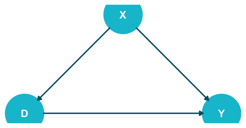
d-Separation tells us whether two variables are conditionally independent given a set \(X\). The backdoor criterion runs that question backwards: given a treatment \(D\) and outcome \(Y\), which \(X\) should we condition on to identify the causal effect \(P(Y \mid do(D))\)? It is the graphical translation of the conditional-exchangeability assumption from potential outcomes — and the rule of thumb that catches the most common adjustment mistakes before they happen.
A backdoor path from \(D\) to \(Y\) is any path that starts with an arrow into \(D\) (i.e., \(D \leftarrow \cdots\)). These are the non-causal channels — confounders and their descendants on the \(D\) side — through which \(D\) and \(Y\) become associated even in the absence of any causal effect. Causal paths, by contrast, follow arrows out of \(D\) toward \(Y\) and represent the genuine effect we want to measure. The job of the backdoor criterion is to block the backdoor paths without disturbing the causal ones.
The two conditions are not redundant. Condition 1 closes the confounding paths; condition 2 keeps us from accidentally adjusting away part of the causal effect. A descendant of \(D\) — including the outcome’s mediators or any post-treatment variable — must not be in \(X\), even if including it would happen to block some backdoor path, because conditioning on a post-treatment variable can also block, or twist, a causal path.
Multiple valid sets. A given DAG often admits several sets that satisfy the criterion. Tools such as dagitty::adjustmentSets() and pgmpy.CausalInference.get_all_backdoor_adjustment_sets() enumerate them. Among them, prefer a minimal sufficient set (no redundant variables), and within that, prefer variables that are (a) well-measured and reliable, (b) have good overlap across treatment groups (the positivity assumption), and (c) are clearly pre-treatment. High-dimensional conditioning sets pump up variance and risk positivity violations, even when they remain technically valid.
Proof: backdoor adjustment formula (3 steps)
Let \(X\) satisfy the backdoor criterion relative to \((D, Y)\).
Step 1 — Law of total probability. Condition on \(X\) and marginalise:
\[P(Y \mid do(D = d)) = \sum_{x} P(Y \mid do(D = d), X = x)\, P(X = x \mid do(D = d)).\]
Step 2 — All backdoor paths blocked (condition 1). Once \(X\) is held fixed, the do-operator on \(D\) behaves like ordinary observation of \(D\) for the outcome \(Y\):
\[P(Y \mid do(D = d), X = x) = P(Y \mid D = d, X = x).\]
Step 3 — No descendants of \(D\) in \(X\) (condition 2). Intervening on \(D\) cannot affect \(X\), since no directed path \(D \to X\) exists:
\[P(X \mid do(D = d)) = P(X).\]
Substituting back into Step 1 yields the backdoor adjustment formula:
\[P(Y \mid do(D = d)) = \sum_{x} P(Y \mid D = d, X = x)\,P(X = x). \quad \text{q.e.d.}\]
4.3.2 The Frontdoor Criterion
The backdoor criterion handles the most common identification scenario: all confounders are observed and measurable. But what if a confounder is unobserved? Then no amount of stratification can recover the effect — the variable you would need to condition on is simply not in your dataset, and no machine-learning algorithm can change that.
The frontdoor criterion (Pearl 2009) is the answer to this exact problem. It identifies \(P(Y \mid do(D))\) via a fully mediating variable \(M\) even when there is an unobserved confounder \(U\) between \(D\) and \(Y\). Consider a textbook example: social-media spend (\(D\)) \(\to\) word-of-mouth reach (\(M\)) \(\to\) sales (\(Y\)), with brand awareness (\(U\)) as an unobserved common cause of \(D\) and \(Y\). Backdoor adjustment is impossible (we cannot condition on \(U\)), but if \(M\) satisfies three structural conditions, the effect is still identified.
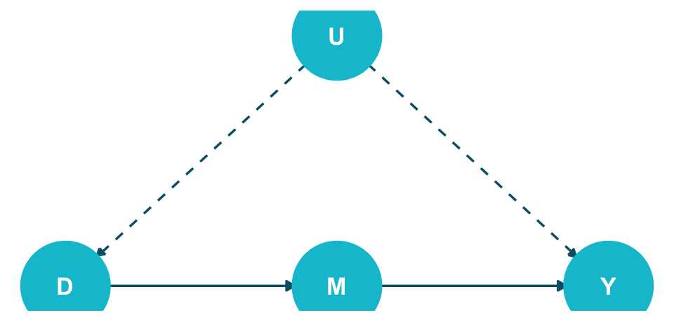
The structural intuition is to split an un-identifiable problem into two identifiable pieces. The effect of \(D\) on \(M\) is identified directly: the only backdoor path \(D \leftarrow U \to Y \leftarrow M\) is blocked by the collider at \(Y\), so \(P(M \mid do(D)) = P(M \mid D)\). The effect of \(M\) on \(Y\) is identified by adjusting for \(D\), which blocks the backdoor \(M \leftarrow D \leftarrow U \to Y\), giving \(P(Y \mid do(M)) = \sum_{d} P(Y \mid M, D = d)\,P(D = d)\). Composing the two pieces by marginalising over \(M\) yields the formula. Full mediation (condition 1) is the strongest of the three assumptions and the most often-violated in practice — most real mediators are partial. When the criterion does hold, however, it is the canonical example of identification despite unobserved confounding, and it shows that the backdoor is not the only weapon in the identification arsenal.
Proof: frontdoor adjustment formula
Setup: a DAG with treatment \(D\), mediator \(M\), outcome \(Y\), and unobserved confounder \(U\), with edges \(U \to D\), \(U \to Y\), \(D \to M\), \(M \to Y\).
Step 1 — Bayesian-network factorisation. The DAG implies
\[P(U, D, M, Y) = P(U)\,P(D \mid U)\,P(M \mid D)\,P(Y \mid U, M).\]
Step 2 — Truncated factorisation under \(do(D = d)\). Intervening on \(D\) removes the factor \(P(D \mid U)\):
\[P(U, M, Y \mid do(D = d)) = P(U)\,P(M \mid D = d)\,P(Y \mid U, M).\]
Step 3 — Marginalise over \(U\):
\[P(M, Y \mid do(D = d)) = P(M \mid D = d)\,\sum_{u} P(Y \mid U = u, M)\,P(U = u).\]
Step 4 — Substitute for \(P(U)\) using \(U \perp\!\!\!\perp M \mid D\):
\[P(U = u) = \sum_{d'} P(U = u \mid D = d', M = m)\,P(D = d').\]
Step 5 — Recognise a conditional joint and use \(Y \perp\!\!\!\perp D \mid U, M\):
\[\sum_{u} P(Y \mid U = u, M = m)\,P(U = u \mid D = d', M = m) = P(Y \mid D = d', M = m).\]
Step 6 — Assemble. Marginalising over \(M\) gives the frontdoor adjustment formula:
\[P(Y \mid do(D = d)) = \sum_{m} P(M = m \mid D = d)\sum_{d'} P(Y \mid M = m, D = d')\,P(D = d'). \quad \text{q.e.d.}\]
4.3.3 do-Calculus and the Causal Hierarchy
The backdoor and frontdoor criteria are two specific identification strategies. The do-calculus (Pearl 2009) is the general identification engine: a complete set of three algebraic rules that systematically convert do-expressions into observational expressions whenever such a conversion is possible. Both backdoor and frontdoor adjustment are theorems of do-calculus; the rules apply far beyond either special case.
The rules use two graph-surgery operations on the original DAG \(G\):
- \(G_{\overline{X}}\): delete every arrow into \(X\) (the surgery of intervention).
- \(G_{\underline{X}}\): delete every arrow out of \(X\) (the surgery that lets us treat \(X\) as conditioned upon, not transmitted from).
Read informally: Rule 1 lets us drop irrelevant observations, Rule 2 lets us turn interventions into observations (the workhorse — this is what “do becomes see” requires), and Rule 3 lets us drop irrelevant interventions. The rules are complete (Shpitser and Pearl 2006): if a causal effect is identifiable from observational data, the rules will find an identifying expression; if they cannot, no method can — additional data (an instrument, an experiment, a new measured variable) is required.
4.3.3.1 Worked example: the college wage premium
A stylised example shows the three rules in concert. Let \(C\) = college degree, \(Y\) = earnings, \(W\) = occupation, \(H\) = work-related health, \(E\) = other socio-economic factors. Dashed bidirected edges represent unobserved confounders: \(Y \leftrightarrow W\) and \(C \leftrightarrow E\). The target is \(P(y \mid do(c))\).
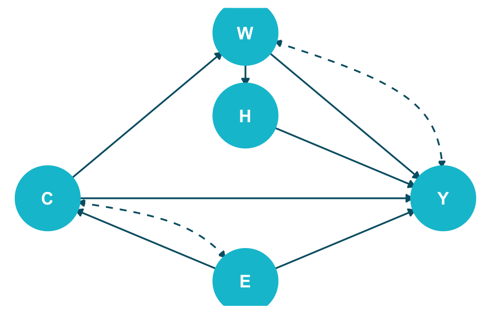
Step 1 — Condition on \(E\) to address the backdoor paths. Two backdoor paths from \(C\) to \(Y\) pass through \(E\). Marginalising over \(E\): \[ P(y \mid do(c)) \;=\; \sum_{e} P(y \mid do(c), e)\, P(e \mid do(c)). \]
Step 2 — Apply Rule 2 to exchange \(do(c)\) for observation. In \(G_{\underline{C}}\) (arrows out of \(C\) deleted), \(C\) and \(Y\) are d-separated given \(E\), so \[ P(y \mid do(c), e) \;=\; P(y \mid c, e) \quad \text{since} \quad Y \perp\!\!\!\perp_{G_{\underline{C}}} C \mid E. \] This is the workhorse step: the interventional quantity becomes an observational conditional.
Step 3 — Apply Rule 3 to drop \(do(c)\) from the marginal of \(E\). In \(G_{\overline{C}}\) (arrows into \(C\) deleted), \(E\) is independent of \(C\), so \[ P(e \mid do(c)) \;=\; P(e) \quad \text{since} \quad E \perp\!\!\!\perp_{G_{\overline{C}}} C. \]
Substituting back yields the fully do-free identifying formula: \[ \boxed{\,P(y \mid do(c)) \;=\; \sum_{e} P(y \mid c, e)\, P(e)\,}. \]
Every quantity on the right-hand side is estimable from observational data. Even with two unobserved confounder edges, the causal effect is identifiable, derived by mechanical application of Rules 2 and 3. This is exactly what software packages such as causaleffect (R) and DoWhy (Python) automate.
4.3.4 Causal Discovery
Everything in the preceding three sections — backdoor, frontdoor, do-calculus — takes the DAG as a given input. The analyst draws the graph from domain knowledge, and the algorithms tell them which adjustments identify the causal effect. But this raises the deeper question: where does the DAG itself come from?
Three honest answers exist. Domain experts draw the graph from substantive knowledge — economists know wages depend on education and ability; doctors know infection precedes symptoms. Randomised experiments establish individual edges by intervention. And, when neither is available at the required scope, causal-discovery algorithms attempt to recover graph structure directly from observational data. This last route — its promise, its assumptions, and its honest limits — is the topic here.
4.3.4.1 What can data alone tell us about the DAG?
Less than students typically expect. Consider three different DAGs over \(\{A, B, C\}\): the chain \(A \to B \to C\), the reverse chain \(A \leftarrow B \leftarrow C\), and the fork \(A \leftarrow B \to C\). All three imply exactly the same conditional independence: \(A \perp\!\!\!\perp C \mid B\), and no other independencies. They are Markov equivalent: no statistical test on observational data can distinguish among them. The fork (a confounder) and the two chains (mediation in either direction) make the same predictions about every conditional probability.
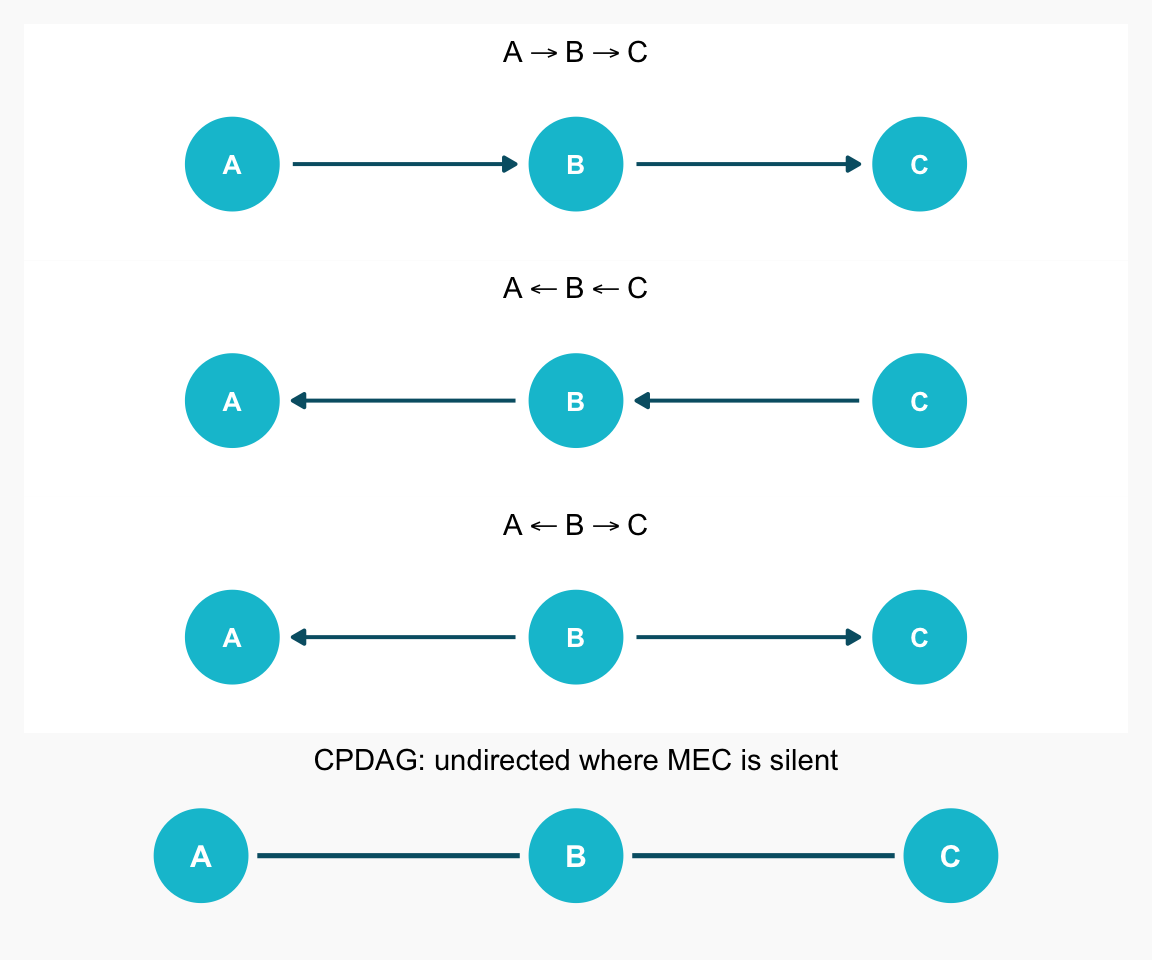
The exception is the collider: \(A \to B \leftarrow C\) implies \(A \perp\!\!\!\perp C\) marginally but \(A \not\perp\!\!\!\perp C \mid B\). Conditioning opens the collider, so its independence pattern is detectable from data — and that breaks the equivalence class. So observational discovery, in general, returns a Markov equivalence class (MEC), summarised graphically as a CPDAG (Completed Partially Directed Acyclic Graph): a graph with directed edges where v-structures and propagation rules pin them down, and undirected edges where the data simply cannot adjudicate. To go further, we need either an additional structural assumption (LiNGAM uses non-Gaussianity) or experimental data.
4.3.4.2 Three families of discovery algorithms
The discovery literature is large, but it organises naturally into three families, each defined by what it uses in the data to recover structure:
| Family | Central question | Output | Key assumption | Examples |
|---|---|---|---|---|
| Constraint-based | Which conditional independencies hold in the data? | CPDAG (or PAG with latents) | Faithfulness | PC, FCI |
| Score-based | Which DAG fits the data best under a score (BIC, BDe)? | CPDAG | Score consistency | GES, GIES |
| Functional / non-Gaussian | Can asymmetries in the noise distribution break the MEC tie? | Unique DAG | Linearity + non-Gaussian noise (or nonlinearity) | LiNGAM, ANM |
We walk PC in detail below — it is the canonical and most-implemented method — and sketch GES, FCI, and LiNGAM at conceptual depth.
4.3.4.3 PC algorithm: skeleton, then orient
PC (Spirtes, Glymour, and Scheines 2000) turns the d-separation criterion backwards: starting from “everything is connected”, it removes edges as conditional independencies are detected, then orients as far as the data and the rules allow. Three phases:
Step 1 — Skeleton. Start with the complete undirected graph on the \(p\) variables. For each pair \((X, Y)\) and every conditioning set \(Z\) of increasing size drawn from the current neighbours of \(X\) or \(Y\), test \(X \perp\!\!\!\perp Y \mid Z\). If any such \(Z\) certifies independence, remove the edge \(X \! - \! Y\) and store \(Z\) as the separating set \(\text{sepset}(X, Y)\). The output is the skeleton: an undirected graph whose edges correspond to pairs that remain dependent under every tested conditioning set.
Step 2 — Orient v-structures. For every unshielded triple \(X \! - \! Z \! - \! Y\) (i.e., \(X\) and \(Y\) are not adjacent in the skeleton), check whether \(Z \in \text{sepset}(X, Y)\). If \(Z \notin \text{sepset}(X, Y)\), the triple must be a v-structure: orient \(X \to Z \leftarrow Y\). The logic: if \(X\) and \(Y\) are independent given a set that excludes \(Z\), then \(Z\) is a collider — conditioning on it would have opened the path, breaking the independence we observed.
Step 3 — Meek’s rules. Propagate orientations using four logical rules that exploit two constraints: acyclicity (no directed cycles allowed) and no new v-structures (any orientation that would create an unshielded collider not already detected in Step 2 is forbidden — that v-structure would have been caught earlier). Repeat until no further edge can be oriented. Edges that remain undirected reflect genuine MEC ambiguity.
4.3.4.4 GES: scoring DAGs instead of testing them
GES (Greedy Equivalence Search; Chickering (2002)) takes a different tack: define a global goodness-of-fit score on DAGs (BIC for Gaussian data, BDe for discrete), then search the space of DAGs greedily for the highest-scoring one. The search proceeds in two phases — a forward phase that adds edges one at a time as long as they improve the score, then a backward phase that removes edges that no longer pull their weight. GES returns a CPDAG, like PC, and is score-consistent: under standard assumptions, the recovered CPDAG converges to the true MEC as \(n \to \infty\). In practice, PC and GES often produce similar CPDAGs but disagree on individual edges; running both and comparing is good hygiene.
4.3.4.5 LiNGAM: non-Gaussianity breaks the tie
LiNGAM (Linear Non-Gaussian Acyclic Model; Shimizu et al. (2006)) trades the MEC limitation for an additional structural assumption. The data are assumed to come from a linear SEM \[X_i = \sum_{j} b_{ij}\,X_j + \varepsilon_i,\] where the noise terms \(\varepsilon_i\) are mutually independent and non-Gaussian. Under that assumption, the unique DAG is identifiable from observational data — not just the equivalence class. The intuition is asymmetry: in the right causal direction, regression residuals retain the non-Gaussian shape of the structural noise; in the wrong direction, they become a difference of two non-Gaussian terms with opposite signs and look symmetric. With Gaussian noise, both directions look the same — that is exactly the MEC limitation. With non-Gaussian noise, the asymmetry is real and statistically detectable. Algorithmically, LiNGAM applies independent component analysis (ICA) to the residuals to estimate the structural-equation matrix \(B\). Generalisations such as ANM (additive noise models) extend the idea to nonlinear functions with additive noise.
4.3.4.6 What discovery does (and doesn’t) deliver
A realistic summary of what students should expect from discovery in 2026:
- It does narrow the space of plausible DAGs from “all of them” to a small equivalence class, often a single CPDAG. This is far more than nothing.
- It does flag edges that domain experts had not considered, prompting useful questions about mechanism.
- It does produce a clean falsifiability test: if the data systematically violate the CIs implied by the expert’s DAG, the expert’s DAG is wrong somewhere.
- It does not give a unique DAG from observational data alone (except under strong assumptions like LiNGAM’s non-Gaussianity).
- It does not distinguish a confounder from a chain or its reverse (the central MEC limitation).
- It does not obviate the need for substantive knowledge or experiments — which sound like limitations but are really design choices: discovery is a hypothesis generator, not an oracle.
Best practice combines all three sources: discovery proposes, expertise edits, and experiments confirm. Where the stakes warrant — a high-cost decision, a regulatory filing, a clinical recommendation — an experiment on at least one critical edge is non-negotiable.
4.4 Coding Lab
4.4.1 Exercise 1: Backdoor Criterion and Adjustment Sets
Difficulty: Applied | Estimated time: 45 minutes
Consider a DAG with 7 variables modelling the effect of a training program (\(D\)) on employee performance (\(Y\)):
- Experience (\(Z_1\)): affects training participation (\(D\)) and performance (\(Y\))
- Department (\(Z_2\)): affects training participation (\(D\)) and motivation (\(Z_3\))
- Motivation (\(Z_3\)): affects performance (\(Y\))
- Skills acquired (\(M\)): mediator, \(D \to M \to Y\)
- Peer evaluation (\(C\)): collider, \(D \to C \leftarrow Y\)
- Training hours (\(W\)): descendant of \(D\), \(D \to W\)
The true causal effect of training on performance is \(\tau = 2.0\) (direct effect only, not through the mediator).
Tasks:
- Draw the DAG and identify all backdoor paths from \(D\) to \(Y\).
- Determine which variable sets satisfy the backdoor criterion. Verify with software.
- Simulate data from this DAG with \(n = 5000\) and compute four estimates:
- Naive (no adjustment)
- Adjusting for a correct minimal set
- Adjusting for the collider \(C\)
- Adjusting for the mediator \(M\)
- Compare all four estimates and explain the direction and magnitude of each bias.
library(dagitty)
library(ggdag)
library(dplyr)

dag <- dagify(
  # Fill in edges from the description
  # ___ ~ ___,
  exposure = "D",
  outcome = "Y",
  coords = list(
    x = c(Z1 = 0, Z2 = 1, D = 0.5, Z3 = 1.5, M = 1, Y = 1.5, C = 1, W = 0),
    y = c(Z1 = 1, Z2 = 1, D = 0.5, Z3 = 0.5, M = 0, Y = 0, C = -0.5, W = 0)
  )
)

# (b) Find adjustment sets
adjustmentSets(dag, type = "minimal")

# (c) Simulate data
set.seed(42)
n <- 5000
# Z1 <- rnorm(n)
# Z2 <- rnorm(n)
# Z3 <- 0.8 * Z2 + rnorm(n, sd = 0.5)
# D  <- rbinom(n, 1, plogis(...))
# M  <- 0.5 * D + rnorm(n, sd = 0.5)
# Y  <- 2.0 * D + ...
# C  <- 0.4 * D + 0.3 * Y + rnorm(n, sd = 0.5)
# W  <- 0.8 * D + rnorm(n, sd = 0.3)

# Compute (i) Naive, (ii) Adjusted (correct), (iii) Collider, (iv) Mediator
import numpy as np
import pandas as pd
from pgmpy.models import BayesianNetwork
from pgmpy.inference import CausalInference
model = BayesianNetwork([
# Fill in edges
])
ci = CausalInference(model)
print(ci.get_all_backdoor_adjustment_sets("D", "Y"))
np.random.seed(42)
n = 5000
# ...
TipShow solution
Show solution
library(dagitty); library(ggdag); library(dplyr)

dag <- dagify(
  D ~ Z1 + Z2,
  Y ~ Z1 + Z3 + M + D,
  Z3 ~ Z2,
  M ~ D,
  C ~ D + Y,
  W ~ D,
  exposure = "D",
  outcome = "Y",
  coords = list(
    x = c(Z1 = 0, Z2 = 1, D = 0.5, Z3 = 1.5, M = 1, Y = 1.5, C = 1, W = 0),
    y = c(Z1 = 1, Z2 = 1, D = 0.5, Z3 = 0.5, M = 0, Y = 0, C = -0.5, W = 0)
  )
)

dag |>
  ggplot(aes(x = x, y = y, xend = xend, yend = yend)) +
  geom_dag_point(colour = "#00C1D4", size = 18) +
  geom_dag_edges(edge_colour = "#005e73", edge_width = 0.8) +
  geom_dag_text(colour = "white", size = 3.5, fontface = "bold") +
  theme_dag()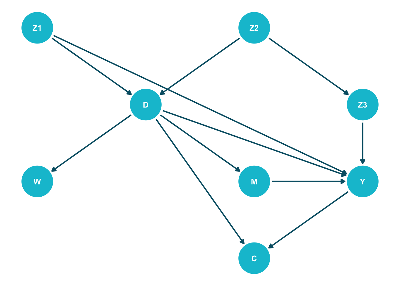
Show solution
# Backdoor paths:
#   1. D <- Z1 -> Y       (fork through Z1)
#   2. D <- Z2 -> Z3 -> Y (chain through Z2, Z3)

cat("Minimal adjustment sets:\n")
Minimal adjustment sets:Show solution
print(adjustmentSets(dag, type = "minimal")){ Z1, Z3 }
{ Z1, Z2 }Show solution
# {Z1, Z2} or {Z1, Z3}

set.seed(42)
n  <- 5000
Z1 <- rnorm(n)
Z2 <- rnorm(n)
Z3 <- 0.8 * Z2 + rnorm(n, sd = 0.5)
D  <- rbinom(n, 1, plogis(0.6 * Z1 + 0.5 * Z2))
M  <- 0.5 * D + rnorm(n, sd = 0.5)
Y  <- 2.0 * D + 1.0 * Z1 + 0.7 * Z3 + 1.0 * M + rnorm(n)
C  <- 0.4 * D + 0.3 * Y + rnorm(n, sd = 0.5)
W  <- 0.8 * D + rnorm(n, sd = 0.3)

df <- tibble(Z1, Z2, Z3, D, M, Y, C, W)

naive       <- mean(df$Y[df$D == 1]) - mean(df$Y[df$D == 0])
adjusted    <- coef(lm(Y ~ D + Z1 + Z2, data = df))["D"]
collider_a  <- coef(lm(Y ~ D + C,        data = df))["D"]
mediator_a  <- coef(lm(Y ~ D + M + Z1 + Z2, data = df))["D"]

cat("(i)   Naive:                ", round(naive,      3), "\n")
(i) Naive: 3.348 Show solution
cat("(ii) Adjusted {Z1, Z2}: ", round(adjusted, 3), "\n")(ii) Adjusted {Z1, Z2}: 2.577 Show solution
cat("(iii) Adjusted for collider:", round(collider_a, 3), "\n")(iii) Adjusted for collider: 1.165 Show solution
cat("(iv) Adjusted for mediator:", round(mediator_a, 3), "\n")(iv) Adjusted for mediator: 2.074 Discussion:
- (i) Naive (~3.5): biased upward; conflates the causal effect of \(D\) with confounding through \(Z_1\) and through \(Z_2 \to Z_3\).
- (ii) Adjusted \(\{Z_1, Z_2\}\) (~2.5): recovers the total causal effect, which is direct (2.0) + indirect through \(M\) (0.5) = 2.5.
- (iii) Adjusted for \(C\) (biased): opens the collider path \(D \to C \leftarrow Y\), introducing a new bias while the original confounding is only partially addressed.
- (iv) Adjusted for \(M\) (~2.0): blocks the indirect path \(D \to M \to Y\), leaving only the direct effect — this is the controlled direct effect, not the total effect that backdoor adjustment targets.
import numpy as np, pandas as pd
import statsmodels.formula.api as smf

np.random.seed(42)
n  = 5000
Z1 = np.random.normal(size=n)
Z2 = np.random.normal(size=n)
Z3 = 0.8 * Z2 + np.random.normal(scale=0.5, size=n)
D  = np.random.binomial(1, 1 / (1 + np.exp(-(0.6 * Z1 + 0.5 * Z2))))
M  = 0.5 * D + np.random.normal(scale=0.5, size=n)
Y  = 2.0 * D + 1.0 * Z1 + 0.7 * Z3 + 1.0 * M + np.random.normal(size=n)
C  = 0.4 * D + 0.3 * Y + np.random.normal(scale=0.5, size=n)
W  = 0.8 * D + np.random.normal(scale=0.3, size=n)

df = pd.DataFrame({"Z1":Z1, "Z2":Z2, "Z3":Z3, "D":D, "M":M, "Y":Y, "C":C, "W":W})

naive   = df.loc[df.D == 1, "Y"].mean() - df.loc[df.D == 0, "Y"].mean()
adj     = smf.ols("Y ~ D + Z1 + Z2", data=df).fit().params["D"]
coll    = smf.ols("Y ~ D + C",        data=df).fit().params["D"]
medi    = smf.ols("Y ~ D + M + Z1 + Z2", data=df).fit().params["D"]

print(f"(i)   Naive:                 {naive:.3f}")
print(f"(ii)  Adjusted (Z1, Z2):     {adj:.3f}")
print(f"(iii) Adjusted for collider: {coll:.3f}")
print(f"(iv)  Adjusted for mediator: {medi:.3f}")
4.4.2 Exercise 2: The Frontdoor Criterion
Difficulty: Challenge | Estimated time: 40 minutes
A company wants to estimate the causal effect of a recommendation algorithm (\(D\), binary: on/off) on purchases (\(Y\), continuous). They suspect that user intent (\(U\)) is an unobserved confounder: users with high purchase intent are more likely to receive recommendations (the algorithm targets them) and more likely to buy regardless. The algorithm’s effect, however, is fully mediated through clicks (\(M\), binary).
The DAG is: \(U \to D\), \(U \to Y\), \(D \to M\), \(M \to Y\).
Tasks:
- Verify that the backdoor criterion cannot be satisfied (no valid adjustment set exists, since \(U\) is unobserved).
- Verify that \(M\) satisfies the frontdoor criterion.
- Simulate data with \(n = 10{,}000\) where the true effect of \(D\) on \(M\) is \(+0.3\) (probability increase) and the true effect of \(M\) on \(Y\) is \(5.0\). Implement the frontdoor estimator.
- Compare: (i) naive (biased by \(U\)), (ii) frontdoor (should recover the truth), (iii) what happens if you incorrectly adjust for \(M\) as a confounder.
library(dagitty); library(dplyr)

dag <- dagify(D ~ U, Y ~ U + M, M ~ D, latent = "U")
adjustmentSets(dag, exposure = "D", outcome = "Y")  # empty: U unobserved

set.seed(123)
n <- 10000
U <- rnorm(n)
D <- rbinom(n, 1, plogis(0.8 * U))
M <- rbinom(n, 1, plogis(-1 + 1.5 * D))
Y <- 5.0 * M + 2.0 * U + rnorm(n)

# Frontdoor: P(Y | do(D=d)) = sum_m P(M=m|D=d) * sum_d' P(Y|M=m,D=d') P(D=d')
# Implement and compare to naive and to adjust-for-M.
import numpy as np, pandas as pd
import statsmodels.formula.api as smf
np.random.seed(123)
n = 10_000
U = np.random.normal(size=n)
D = np.random.binomial(1, 1 / (1 + np.exp(-(0.8 * U))))
M = np.random.binomial(1, 1 / (1 + np.exp(-(-1 + 1.5 * D))))
Y = 5.0 * M + 2.0 * U + np.random.normal(size=n)
df = pd.DataFrame({"U":U, "D":D, "M":M, "Y":Y})
# Implement the frontdoor formula and compare estimates.4.4.3 Exercise 3: Causal Discovery on a Simulated 5-Node SEM
Difficulty: Challenge | Estimated time: 40 minutes
This exercise mirrors the lecture’s PC walkthrough on a 5-node linear SEM and lets you compare the three discovery families on the same data. The data-generating process:
- \(A\) and \(B\) are root nodes drawn from \(\mathcal{N}(0, 1)\) (or a non-Gaussian gamma — see (b))
- \(C = 0.7\,A + \varepsilon_C\)
- \(D = 0.6\,A + 0.6\,B + 0.5\,C + \varepsilon_D\) (a 3-parent collider)
- \(E\) is an isolated decoy node, same noise, no edges
The true (oriented) DAG: \(A \to C\), \(A \to D\), \(B \to D\), \(C \to D\); \(E\) has no edges. The CPDAG that PC should recover under faithful CIs has the v-structure at \(D\) identified (\(A,B,C \to D\)) and the \(A \! - \! C\) edge undirected (the two orientations \(A \to C\) and \(C \to A\) are Markov-equivalent here).
Tasks:
- Simulate \(n = 1000\) observations from the SEM with Gaussian noise. Run the PC algorithm and inspect the CPDAG. Verify that the v-structure at \(D\) is recovered and that the \(A \! - \! C\) edge is left undirected.
- Repeat with non-Gaussian (gamma) noise: replace \(\mathcal{N}(0, 1)\) with a centred Gamma(2, 1) draw, \(\text{rgamma}(n, 2, 1) - 2\). Run LiNGAM on the same data; verify that \(A \to C\) is now oriented uniquely.
- Run GES on the Gaussian-noise data. Compare the GES CPDAG with PC’s. Where do they agree? Where do they disagree?
- Re-run PC at three significance levels (\(\alpha = 0.01, 0.05, 0.10\)). Document how the recovered skeleton changes. What does this tell you about reading any single discovery output as “the” graph?
# install.packages(c("pcalg", "graph", "Rgraphviz"))   # graph/Rgraphviz via BiocManager

library(pcalg)

simulate_sem <- function(n, gaussian = TRUE) {
  noise <- if (gaussian) rnorm else \(k) rgamma(k, 2, 1) - 2
  A <- noise(n);  B <- noise(n)
  C <- 0.7 * A + noise(n)
  D <- 0.6 * A + 0.6 * B + 0.5 * C + noise(n)
  E <- noise(n)
  data.frame(A, B, C, D, E)
}

set.seed(7)
df_g <- simulate_sem(1000, gaussian = TRUE)

# (a) PC on Gaussian data
pc_g <- pc(suffStat = list(C = cor(df_g), n = nrow(df_g)),
           indepTest = gaussCItest, alpha = 0.05,
           labels = colnames(df_g))
plot(pc_g, main = "PC CPDAG, Gaussian noise")

# (b) LiNGAM on non-Gaussian data
df_ng <- simulate_sem(1000, gaussian = FALSE)
li <- lingam(as.matrix(df_ng))
print(li$Bpruned)   # nonzero entries give oriented edges

# (c) GES on Gaussian data
ges_g <- ges(new("GaussL0penObsScore", df_g))
plot(ges_g$essgraph, main = "GES CPDAG")

# (d) Sensitivity sweep over alpha
for (a in c(0.01, 0.05, 0.10)) {
  pc_a <- pc(suffStat = list(C = cor(df_g), n = nrow(df_g)),
             indepTest = gaussCItest, alpha = a,
             labels = colnames(df_g))
  cat("alpha =", a, ": adjacency =\n"); print(as(pc_a, "amat"))
}
# pip install causal-learn lingam matplotlib pydot
import numpy as np
import pandas as pd
from causallearn.search.ConstraintBased.PC import pc
from causallearn.search.ScoreBased.GES import ges
import lingam
def simulate_sem(n, gaussian=True, rng=None):
rng = rng or np.random.default_rng(7)
noise = (lambda k: rng.standard_normal(k)) if gaussian \
else (lambda k: rng.gamma(2, 1, k) - 2)
A = noise(n); B = noise(n)
C = 0.7 * A + noise(n)
D = 0.6 * A + 0.6 * B + 0.5 * C + noise(n)
E = noise(n)
return pd.DataFrame({"A":A, "B":B, "C":C, "D":D, "E":E})
# (a) PC on Gaussian data
df_g = simulate_sem(1000, gaussian=True)
cg = pc(df_g.values, alpha=0.05, indep_test="fisherz", node_names=list(df_g))
cg.draw_pydot_graph()
# (b) LiNGAM on non-Gaussian data
df_ng = simulate_sem(1000, gaussian=False)
m = lingam.DirectLiNGAM().fit(df_ng.values)
print(m.adjacency_matrix_)
# (c) GES on Gaussian data
ges_res = ges(df_g.values, score_func="local_score_BIC", node_names=list(df_g))
print(ges_res["G"])
# (d) Sensitivity sweep over alpha
for a in [0.01, 0.05, 0.10]:
cg_a = pc(df_g.values, alpha=a, indep_test="fisherz", node_names=list(df_g))
print(f"alpha={a}: edges =\n", cg_a.G.graph)4.4.4 Exercise 4: Capstone — Integrated Workflow on the Lalonde Job Training Data
Difficulty: Capstone | Estimated time: 75 minutes
This capstone walks the full causal-graph pipeline end to end on a single dataset: scenario → DAG specification → causal discovery → identification (backdoor + frontdoor + general do-calculus) → critical reflection. Every concept introduced in this session and Session 02 shows up at least once. Read the prose, run the R chunks, then verify with the Python tabs.
4.4.4.1 Step 1 — The dataset and scenario
The Lalonde dataset comes from a job-training program designed to test whether training causally raises future earnings. The observed variables are:
- Education (
edu, years of schooling), - Age (
age, years), - Prior earnings (
prior, average annual earnings before training), - Future earnings (
earn, annual earnings after training, our outcome), - Job training (
train, our binary treatment).
Three plausibly relevant variables are not in the data and act as latent: a single bundle of socio-economic background factors (parental education, neighbourhood, network, motivation), a measurable skill acquisition test that could have been given right after the training, and a quality-of-CV rating (“resume strength”) used in subsequent applications. To make the DAG mechanism concrete and to give the discovery algorithm something to recover, we simulate skill and resume from the observed variables and rebuild earn from a known structural equation.
library(Matching)   # contains the lalonde dataset
library(tidyverse)  # data wrangling
library(Hmisc)      # cut2() for equal-frequency binning

set.seed(11)
data(lalonde)

dat <- lalonde |>
  mutate(prior = (re75 + re74) / 2) |>                   # average prior earnings
  dplyr::select(age, edu = educ, prior, train = treat, earn = re78) |>
  mutate(
    # skill <- training + a bit of education (unobserved at first)
    skill  = 0.8 * train + 0.3 * as.numeric(scale(edu)) + rnorm(n(), 0, 0.5),
    # resume <- skill + education + prior earnings
    resume = 0.5 * skill + 0.2 * as.numeric(scale(edu)) + 0.5 * prior + rnorm(n(), 0, 0.5),
    # discretise into 5-point ratings (closer to a real measurement)
    skill  = as.integer(Hmisc::cut2(skill,  g = 5)),
    resume = as.integer(Hmisc::cut2(resume, g = 5)),
    # earn <- education + skill + resume + prior earnings (NO direct effect of train!)
    earn   = 0.3 * as.numeric(scale(edu)) +
             5000 * skill + 3000 * resume + 0.6 * prior + rnorm(n(), 0, 0.5)
  )

# write a copy for the Python tab
dir.create("../../materials/data", showWarnings = FALSE, recursive = TRUE)
readr::write_csv(dat, "../../materials/data/lalonde_capstone.csv")

head(dat, 4)
age edu prior train earn skill resume
1 37 11 0 1 29000.56 4 3
2 22 9 0 1 25999.52 4 2
3 30 12 0 1 24001.15 3 3
4 27 11 0 1 18000.62 3 1import numpy as np, pandas as pd
dat = pd.read_csv("../../materials/data/lalonde_capstone.csv")
dat.head(4)| age | edu | prior | train | earn | skill | resume | |
|---|---|---|---|---|---|---|---|
| 0 | 37 | 11 | 0.0 | 1 | 29000.562492 | 4 | 3 |
| 1 | 22 | 9 | 0.0 | 1 | 25999.523273 | 4 | 2 |
| 2 | 30 | 12 | 0.0 | 1 | 24001.151292 | 3 | 3 |
| 3 | 27 | 11 | 0.0 | 1 | 18000.620256 | 3 | 1 |
4.4.4.2 Step 2 — Specify a candidate DAG
Before we look at the data, we draw the DAG we believe describes the world. The candidate has three blocks:
- Confounders of
trainandearn:age,edu,prior— all three plausibly raise both the probability of enrolling in training (mid-career professionals retrain less, more-educated people self-select into more training, low-earners are likelier to seek a programme) and future earnings (seniority, skill premium, autoregression). - Latent socio-economic background
U: raises education, prior earnings, and training take-up (Oreopoulos & Petronijevic 2013); not directly observed. - Mediators:
skill←train(the central training-effect channel of Card 1999);resume←skill + edu + prior(resume strength reflects skill plus paper credentials and prior labour-market history).
library(ggdag); library(dagitty); library(dplyr); library(ggplot2)

coords_dag <- tribble(
  ~name,    ~x, ~y,
  "age",     3, 3.5,
  "edu",     1, 5,
  "prior",   5, 5,
  "U",       3, 6,    # latent background
  "train",   1, 3.5,
  "earn",    5, 3.5,
  "skill",   2, 1.5,
  "resume",  4, 1.5
)

dag <- dagify(
  train  ~ age + edu + prior + U,
  earn   ~ age + edu + prior + skill + resume,
  skill  ~ train,
  prior  ~ U + age + edu,
  edu    ~ U + age,
  resume ~ skill + prior + edu,
  exposure = "train", outcome = "earn",
  latent   = "U",
  coords   = coords_dag
)

dag |>
  tidy_dagitty() |>
  node_status() |>
  ggplot(aes(x = x, y = y, xend = xend, yend = yend)) +
  geom_dag_edges(edge_colour = "#005e73", edge_width = 0.8) +
  geom_dag_point(aes(colour = status), size = 18) +
  geom_dag_text(colour = "white", size = 3.2, fontface = "bold") +
  scale_colour_manual(values = c(exposure = "#FF7E15", outcome = "#005e73",
                                 latent   = "grey50"),
                      na.value = "#00C1D4") +
  guides(colour = "none") +
  theme_dag()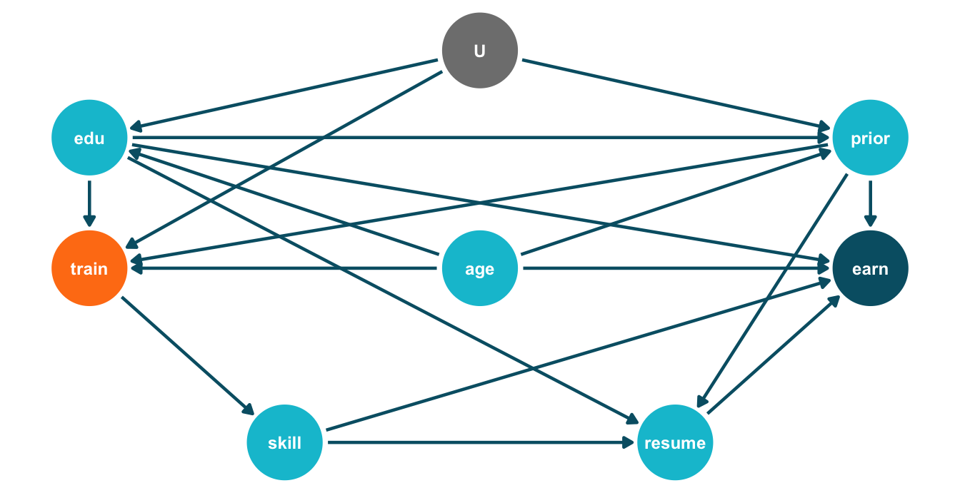
import networkx as nx, matplotlib.pyplot as plt

edges = [("age","train"), ("edu","train"), ("prior","train"), ("U","train"),
         ("age","earn"),  ("edu","earn"),  ("prior","earn"),
         ("skill","earn"), ("resume","earn"),
         ("train","skill"),
         ("U","prior"), ("age","prior"), ("edu","prior"),
         ("U","edu"),   ("age","edu"),
         ("skill","resume"), ("prior","resume"), ("edu","resume")]
pos = {"age":(3,3.5), "edu":(1,5), "prior":(5,5), "U":(3,6),
       "train":(1,3.5), "earn":(5,3.5), "skill":(2,1.5), "resume":(4,1.5)}
roles = {n:("exposure" if n=="train" else "outcome" if n=="earn"
            else "latent" if n=="U" else "other") for n in pos}
colours = {"exposure":"#FF7E15","outcome":"#005e73",
           "latent":"grey","other":"#00C1D4"}

G = nx.DiGraph(edges)
fig, ax = plt.subplots(figsize=(7, 3.6))
_ = nx.draw_networkx_edges(G, pos, ax=ax, edge_color="#005e73", width=1.4,
                           arrowsize=14, node_size=1200)
_ = nx.draw_networkx_nodes(G, pos, ax=ax, node_size=1200,
                           node_color=[colours[roles[n]] for n in G.nodes])
_ = nx.draw_networkx_labels(G, pos, ax=ax, font_color="white",
                            font_size=8, font_weight="bold")
ax.set_axis_off()
plt.tight_layout()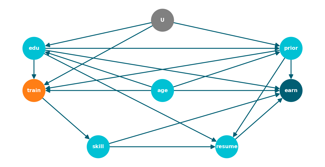
4.4.4.3 Step 3 — Causal Discovery (PC algorithm)
We pretend we don’t know the DAG and let the PC algorithm propose one from the data. PC sees all observed variables (age, edu, prior, train, earn, skill, resume) but not U.
library(pcalg)

obs <- dat[, c("age", "edu", "prior", "train", "earn", "skill", "resume")]
suff <- list(C = cor(obs), n = nrow(obs))
pc_fit <- pc(suff, indepTest = gaussCItest, alpha = 0.05, labels = colnames(obs))
plot(pc_fit, main = "")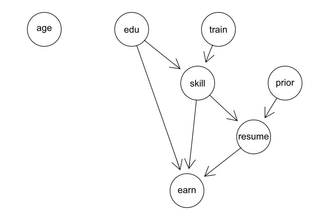
from causallearn.search.ConstraintBased.PC import pc
from causallearn.utils.cit import fisherz

cols = ["age","edu","prior","train","earn","skill","resume"]
X = dat[cols].to_numpy(dtype=float)
cg = pc(X, alpha=0.05, indep_test=fisherz, show_progress=False, node_names=cols)

# Print recovered edges
G = cg.G
out = []
for i in range(G.graph.shape[0]):
    for j in range(i+1, G.graph.shape[0]):
        a, b = G.graph[i, j], G.graph[j, i]
        if a == 0 and b == 0: continue
        # causal-learn convention: graph[i,j]=-1, graph[j,i]=1 means i -> j
        if a == -1 and b == 1:  out.append(f"{cols[i]} -> {cols[j]}")
        elif a == 1 and b == -1: out.append(f"{cols[j]} -> {cols[i]}")
        elif a == -1 and b == -1: out.append(f"{cols[i]} -- {cols[j]}")
print("\n".join(out))
edu -> earn
edu -> skill
prior -- resume
train -> skill
skill -> earn
resume -> earn
resume -> skillPC’s CPDAG agrees with our candidate on most edges, but it makes two corrections worth noting:
- It detects an
edu → skilledge that we did not draw. That is correct: our simulation hasskill = 0.8·train + 0.3·scale(edu) + ε, so education does enter the skill mechanism — the candidate DAG was misspecified on this edge, and PC picked it up. - It drops the direct
age → earnandage → trainconnections in the simulated half (age was inherited only from the real Lalonde records and has no role in the structural equations).
The simplified DAG below reflects the discovery output. The train ↔︎ edu, train ↔︎ prior, edu ↔︎ prior bidirected edges encode the latent U, which now confounds these three variables (PC sees only their correlations, not the common parent).
dag2 <- dagify(
  earn   ~ edu + skill + resume,
  train  ~ U,
  skill  ~ train + edu,        # NEW edge from PC
  prior  ~ U,
  edu    ~ U,
  resume ~ skill + prior,
  exposure = "train", outcome = "earn",
  latent   = "U",
  coords   = filter(coords_dag, name != "age")
)

dag2 |>
  tidy_dagitty() |>
  node_status() |>
  ggplot(aes(x = x, y = y, xend = xend, yend = yend)) +
  geom_dag_edges(edge_colour = "#005e73", edge_width = 0.8) +
  geom_dag_point(aes(colour = status), size = 18) +
  geom_dag_text(colour = "white", size = 3.2, fontface = "bold") +
  scale_colour_manual(values = c(exposure = "#FF7E15", outcome = "#005e73",
                                 latent   = "grey50"),
                      na.value = "#00C1D4") +
  guides(colour = "none") +
  theme_dag()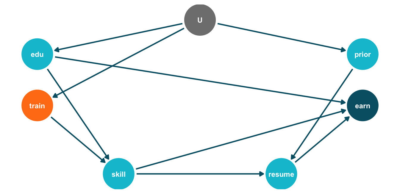
edges2 = [("U","train"),
          ("edu","earn"), ("edu","skill"),
          ("train","skill"),
          ("skill","earn"), ("resume","earn"),
          ("U","prior"), ("U","edu"),
          ("skill","resume"), ("prior","resume")]
pos2 = {k:v for k,v in pos.items() if k != "age"}
G2 = nx.DiGraph(edges2)
fig, ax = plt.subplots(figsize=(7, 3.4))
_ = nx.draw_networkx_edges(G2, pos2, ax=ax, edge_color="#005e73",
                           width=1.4, arrowsize=14, node_size=1200)
_ = nx.draw_networkx_nodes(G2, pos2, ax=ax, node_size=1200,
                           node_color=[colours[roles.get(n,"other")] for n in G2.nodes])
_ = nx.draw_networkx_labels(G2, pos2, ax=ax, font_color="white",
                            font_size=8, font_weight="bold")
ax.set_axis_off()
plt.tight_layout()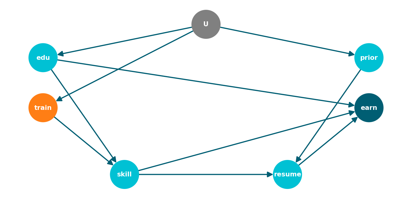
4.4.4.4 Step 4a — Identification: the backdoor criterion
The minimal sufficient adjustment set in the original DAG:
dagitty::adjustmentSets(dag, exposure = "train", outcome = "earn"){ age, edu, prior }from pgmpy.inference import CausalInference
from pgmpy.base import DAG as PGMDAG
g_orig = PGMDAG([("age","train"),("edu","train"),("prior","train"),("U","train"),
("age","earn"),("edu","earn"),("prior","earn"),
("skill","earn"),("resume","earn"),("train","skill"),
("U","prior"),("age","prior"),("edu","prior"),
("U","edu"),("age","edu"),
("skill","resume"),("prior","resume"),("edu","resume")],
latents={"U"})
ci = CausalInference(g_orig)
ci.get_all_backdoor_adjustment_sets("train", "earn")frozenset({frozenset({'edu', 'prior', 'age'})}){age, edu, prior} in both. Now check that resume should not be added: it is a descendant of training and a collider on the path train ← edu → resume ← skill → earn; conditioning on it opens that backdoor.
dagitty::isAdjustmentSet(
  dag, c("age", "edu", "prior", "resume"),
  exposure = "train", outcome = "earn"
)
[1] FALSEimport networkx as nx
# Heads up: pgmpy's is_valid_backdoor_adjustment_set silently *omits* the
# "Z must contain no descendants of X" half of the backdoor criterion --- and
# its d-separation check on the proper-backdoor graph misses the collider that
# `resume` opens here. We therefore check both halves explicitly.
def is_valid_backdoor(graph, ci, X, Y, Z):
if Z & nx.descendants(graph, X):
return False, f"rejected: contains descendant(s) of {X}: {Z & nx.descendants(graph, X)}"
if not ci.is_valid_backdoor_adjustment_set(X, Y, Z=frozenset(Z)):
return False, "rejected: a backdoor path is still open"
return True, "valid"
is_valid_backdoor(g_orig, ci, "train", "earn", {"age","edu","prior","resume"})(False, "rejected: contains descendant(s) of train: {'resume'}")For the simplified DAG discovered by PC:
dagitty::adjustmentSets(dag2, exposure = "train", outcome = "earn"){ edu, prior }g2 = PGMDAG([("U","train"),
("edu","earn"),("edu","skill"),
("train","skill"),
("skill","earn"),("resume","earn"),
("U","prior"),("U","edu"),
("skill","resume"),("prior","resume")],
latents={"U"})
ci2 = CausalInference(g2)
ci2.get_all_backdoor_adjustment_sets("train", "earn")frozenset({frozenset({'edu', 'prior'})}){edu, prior}. We still need both, even though direct edu → train and prior → train edges are gone — the latent U still confounds train with edu and prior.
4.4.4.5 Step 4b — Identification: the frontdoor criterion
Three conditions for the frontdoor through skill:
skillmediates all causal paths fromtraintoearn. ✓ in both DAG variants.- No unblocked backdoor from
traintoskill. - All backdoors from
skilltoearnare blocked bytrain.
# Condition 2: train -> skill (which set, if any, blocks backdoors?)
cat("dag  (train -> skill): "); print(dagitty::adjustmentSets(dag,  "train", "skill"))
dag (train -> skill): {}cat("dag2 (train -> skill): "); print(dagitty::adjustmentSets(dag2, "train", "skill"))dag2 (train -> skill): { edu }# Condition 3: skill -> earn (does {train} block all backdoors?)
cat("dag (skill -> earn): "); print(dagitty::adjustmentSets(dag, "skill", "earn"))dag (skill -> earn): { age, edu, prior }
{ train }cat("dag2 (skill -> earn): "); print(dagitty::adjustmentSets(dag2, "skill", "earn"))dag2 (skill -> earn): { edu, prior }
{ edu, train }# pgmpy quirk: get_all_backdoor_adjustment_sets returns frozenset() (empty)
# when the empty set itself is a valid adjustment, so we also check explicitly.
print("dag (train -> skill): empty set valid?",
ci.is_valid_backdoor_adjustment_set("train","skill", frozenset()))dag (train -> skill): empty set valid? Trueprint("dag2 (train -> skill):", ci2.get_all_backdoor_adjustment_sets("train","skill"))dag2 (train -> skill): frozenset({frozenset({'edu'})})print("dag (skill -> earn):", ci.get_all_backdoor_adjustment_sets("skill","earn"))dag (skill -> earn): frozenset({frozenset({'edu', 'prior', 'age'}), frozenset({'train'})})print("dag2 (skill -> earn):", ci2.get_all_backdoor_adjustment_sets("skill","earn"))dag2 (skill -> earn): frozenset({frozenset({'edu', 'prior'}), frozenset({'train', 'edu'})})In the original DAG, condition 2 is met by the empty set (resume and earn are colliders that block backdoors automatically), and {train} is one valid blocker for condition 3 → frontdoor identification works.
In the simplified DAG, condition 2 requires {edu} (so the backdoor train ← U → edu → skill must be closed) and condition 3 requires {edu, train} together. Once we need edu for condition 2, the strict frontdoor criterion (no other adjustment beyond the mediator) is violated — PC’s discovery has effectively removed the frontdoor route.
4.4.4.6 Step 4c — General do-calculus
Now suppose U also directly affects earn (think of motivation, which both drives training take-up and pays off later in earnings independently of the skill channel). The modified DAG adds one new arrow U → earn (highlighted in orange below) on top of the original structure:
dag_mod <- dagify(
  train  ~ age + edu + prior + U,
  earn   ~ age + edu + prior + skill + resume + U,    # <-- U -> earn is new
  skill  ~ train,
  prior  ~ U + age + edu,
  edu    ~ U + age,
  resume ~ skill + prior + edu,
  exposure = "train", outcome = "earn",
  latent   = "U",
  coords   = coords_dag
)

dag_mod_tidy <- dag_mod |> tidy_dagitty() |> node_status() |>
  dplyr::mutate(new_edge = (name == "U" & to == "earn"))

ggplot(dag_mod_tidy, aes(x = x, y = y, xend = xend, yend = yend)) +
  ggdag::geom_dag_edges_link(
    aes(edge_colour = new_edge),
    edge_width = 0.9,
    arrow = grid::arrow(length = grid::unit(5, "pt"), type = "closed")
  ) +
  geom_dag_point(aes(colour = status), size = 18) +
  geom_dag_text(colour = "white", size = 3.2, fontface = "bold") +
  ggraph::scale_edge_colour_manual(
    values = c(`TRUE` = "#FF7E15", `FALSE` = "#005e73"), guide = "none"
  ) +
  scale_colour_manual(
    values = c(exposure = "#FF7E15", outcome = "#005e73", latent = "grey50"),
    na.value = "#00C1D4"
  ) +
  guides(colour = "none") +
  theme_dag()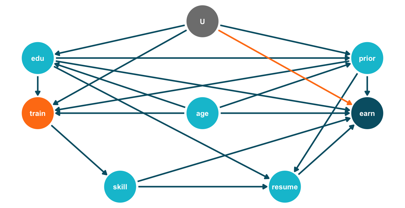
edges_mod = edges + [("U","earn")]   # one new arrow
G_mod = nx.DiGraph(edges_mod)
edge_colours_mod = ["#FF7E15" if e == ("U","earn") else "#005e73"
                    for e in G_mod.edges]
edge_widths = [2.4 if e == ("U","earn") else 1.4 for e in G_mod.edges]

fig, ax = plt.subplots(figsize=(7, 3.6))
_ = nx.draw_networkx_edges(G_mod, pos, ax=ax, edge_color=edge_colours_mod,
                           width=edge_widths, arrowsize=14, node_size=1200)
_ = nx.draw_networkx_nodes(G_mod, pos, ax=ax, node_size=1200,
                           node_color=[colours[roles[n]] for n in G_mod.nodes])
_ = nx.draw_networkx_labels(G_mod, pos, ax=ax, font_color="white",
                            font_size=8, font_weight="bold")
ax.set_axis_off()
plt.tight_layout()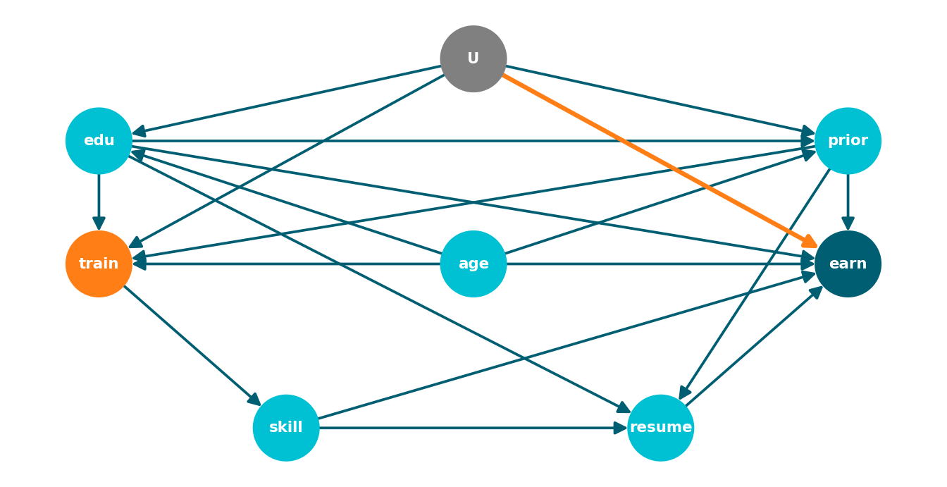
In the corresponding ADMG, the latent U produces three additional bidirected edges against earn: train ↔︎ earn, edu ↔︎ earn, prior ↔︎ earn (in addition to the three pre-existing bidirected edges among train, edu, prior). Backdoor adjustment cannot close all of these with observed variables alone — can the do-calculus still identify the effect?
library(dosearch)

g_admg <- "
  age -> train
  edu -> train
  prior -> train
  age -> earn
  edu -> earn
  prior -> earn
  skill -> earn
  resume -> earn
  train -> skill
  age -> prior
  edu -> prior
  age  -> edu
  skill -> resume
  prior -> resume
  edu   -> resume
  train <-> earn
  train <-> prior
  train <-> edu
  edu <-> prior
  edu <-> earn
  prior <-> earn
"

data_str <- "P(age,edu,prior,train,skill,earn,resume)"
query    <- "P(earn|do(train))"
res <- dosearch(data_str, query, g_admg)

cat("Identifiable: ", is_identifiable(res), "\n\n", sep = "")
Identifiable: TRUE
cat("$$\n", res$formula, "\n$$\n", sep = "")\[ \sum_{skill,prior,edu,age}\left(p(skill|train)\sum_{train}\left(p(train,prior,edu,age)p(earn|train,skill,prior,edu,age)\right)\right) \]
# Python note: there is no exact equivalent of dosearch in the standard
# Python causal-inference stack. dowhy.CausalModel.identify_effect()
# can identify effects that are reducible to backdoor / frontdoor /
# IV adjustments, but it does not return the closed-form formula for
# arbitrary semi-Markovian (bidirected-edge) graphs the way dosearch does.
#
# For the general ID-algorithm in Python, the closest packages are
#   - ananke-causal      (cleanest API; needs older Python)
#   - y0                 (active development; complete ID + IDC)
# Refer to the R block above for the closed-form expression on this DAG.
The closed-form expression returned by dosearch is the frontdoor formula, extended so that condition 3 conditions on train, age, edu, prior together (since U now connects all three to earn). In words: estimate \(P(\text{skill} \mid \text{train})\) from the training mechanism, then average \(P(\text{earn} \mid \text{skill}, \text{train}, \text{age}, \text{edu}, \text{prior})\) over the joint of (train, age, edu, prior) drawn from the observational marginal — a textbook do-calculus identification.
4.4.4.6.1 Estimating the do-calculus formula from data
We now plug data into the formula and compare against the naïve and backdoor-adjusted estimates of the ATE \(E[\text{earn} \mid do(\text{train}=1)] - E[\text{earn} \mid do(\text{train}=0)]\). The formula has two ingredients:
- Mediator law \(P(\text{skill} \mid \text{train})\) — estimated as the empirical conditional distribution of the integer-binned
skillgiventrain. - Outcome regression \(E[\text{earn} \mid \text{train}, \text{skill}, \text{age}, \text{edu}, \text{prior}]\) — estimated by a linear model.
We then sweep over skill levels, weight by the mediator law, and average the predicted earnings over the empirical joint of (train, age, edu, prior) — exactly what the formula prescribes.
# (i) Empirical P(skill | train)
p_skill_given_train <- prop.table(
  table(skill = dat$skill, train = dat$train), margin = 2
)

# (ii) Outcome regression including a train:skill interaction (allows the
#      mediator to carry train-specific effects)
m_earn <- lm(earn ~ train * skill + age + edu + prior, data = dat)

# Plug the two ingredients into the formula
do_train <- function(t_star) {
  total <- 0
  for (s in sort(unique(dat$skill))) {
    p_s <- p_skill_given_train[as.character(s), as.character(t_star)]
    pred <- predict(m_earn, newdata = transform(dat, skill = s))
    total <- total + p_s * mean(pred)
  }
  total
}

ate_do    <- do_train(1) - do_train(0)
ate_bd    <- coef(lm(earn ~ train + age + edu + prior, data = dat))[["train"]]
ate_naive <- coef(lm(earn ~ train,                     data = dat))[["train"]]

cat(sprintf("ATE  do-calculus (frontdoor formula):   %8.0f\n", ate_do))
ATE do-calculus (frontdoor formula): 9376cat(sprintf("ATE backdoor adjustment: %8.0f\n", ate_bd))ATE backdoor adjustment: 8960cat(sprintf("ATE naive (train only): %8.0f\n", ate_naive))ATE naive (train only): 9707import numpy as np
from statsmodels.formula.api import ols
# (i) Empirical P(skill | train), as a (skill, train) table
p_skill_given_train = (
dat.groupby("train")["skill"]
.value_counts(normalize=True).unstack(fill_value=0).T
)
# (ii) Outcome regression with a train:skill interaction
m_earn = ols("earn ~ train * skill + age + edu + prior", data=dat).fit()
def do_train(t_star):
total = 0.0
for s in sorted(dat["skill"].unique()):
p_s = p_skill_given_train.loc[s, t_star]
nd = dat.assign(skill=s)
total += p_s * m_earn.predict(nd).mean()
return total
ate_do = do_train(1) - do_train(0)
ate_bd = ols("earn ~ train + age + edu + prior", data=dat).fit().params["train"]
ate_naive = ols("earn ~ train", data=dat).fit().params["train"]
print(f"ATE do-calculus (frontdoor formula): {ate_do:8.0f}")ATE do-calculus (frontdoor formula): 9376print(f"ATE backdoor adjustment: {ate_bd:8.0f}")ATE backdoor adjustment: 8960print(f"ATE naive (train only): {ate_naive:8.0f}")ATE naive (train only): 97074.4.4.7 Step 5 — Reflection
| DAG variant | Backdoor? | Frontdoor? | Do-calculus identifiable? |
|---|---|---|---|
Original (latent \(U\) confounds train ~ edu ~ prior only) |
✓ via \(\{age, edu, prior\}\) | ✓ via skill (cond. on \(\{train\}\)) |
✓ (reduces to backdoor) |
| Simplified (PC output, same latent \(U\)) | ✓ via \(\{edu, prior\}\) | ✗ (cond. 2 + 3 require \(edu\)) | ✓ (reduces to backdoor) |
| Original + \(U \to \text{earn}\) (no observed backdoor closes) | ✗ | ✓ extended with \(\{train, age, edu, prior\}\) | ✓ |
| Simplified + \(U \to \text{earn}\) + \(edu \to skill\) | ✗ | ✗ | ✓ via a longer do-calculus expression |
4.5 References & Resources
4.5.1 Academic Literature
- Pearl, J. (2009). Causality: Models, Reasoning, and Inference. 2nd ed. Cambridge University Press. — The foundational reference. Chapter 3 covers the do-operator; §3.3 covers backdoor and frontdoor; §3.4 contains the do-calculus rules.
- Pearl, J., Glymour, M. & Jewell, N. P. (2016). Causal Inference in Statistics: A Primer. Wiley. — Chapters 3–4 cover backdoor / frontdoor / do-calculus at an accessible level.
- Pearl, J. (1995). Causal Diagrams for Empirical Research. Biometrika, 82(4), 669–688. — Original publication of the frontdoor criterion.
- Shpitser, I. & Pearl, J. (2006). Identification of Joint Interventional Distributions in Recursive Semi-Markovian Causal Models. AAAI, 1219–1226. — Completeness of do-calculus and the ID algorithm.
- Bareinboim, E., Correa, J. D., Ibeling, D. & Icard, T. (2022). On Pearl’s Hierarchy and the Foundations of Causal Inference. In Probabilistic and Causal Inference: The Works of Judea Pearl. ACM, 507–556. — Comprehensive treatment of Pearl’s Causal Hierarchy and the Causal Hierarchy Theorem.
- Cinelli, C., Forney, A. & Pearl, J. (2022). A Crash Course in Good and Bad Controls. Sociological Methods & Research, 51(3), 1071–1104. — Concise guide to the four adjustment mistakes and their graphical diagnosis.
- Spirtes, P., Glymour, C. & Scheines, R. (2000). Causation, Prediction, and Search. 2nd ed. MIT Press. — The reference for constraint-based discovery (PC and FCI).
- Chickering, D. M. (2002). Optimal Structure Identification with Greedy Search. Journal of Machine Learning Research, 3, 507–554. — The GES paper.
- Shimizu, S., Hoyer, P. O., Hyvärinen, A. & Kerminen, A. (2006). A Linear Non-Gaussian Acyclic Model for Causal Discovery. Journal of Machine Learning Research, 7, 2003–2030. — The LiNGAM paper.
- Glymour, C., Zhang, K. & Spirtes, P. (2019). Review of Causal Discovery Methods Based on Graphical Models. Frontiers in Genetics, 10, 524. — Modern review of the discovery literature.
- Hünermund, P. & Bareinboim, E. (2023). Causal Inference and Data Fusion in Econometrics. The Econometrics Journal, 26(1), 1–34. — Bridges PO and DAG frameworks.
4.5.2 Practitioner Resources
- DAGitty — Interactive web tool for drawing DAGs and finding adjustment sets. Indispensable for both Exercises 1 and 2.
- Tennant, P. W. G. et al. (2021). Use of Directed Acyclic Graphs (DAGs) to Identify Confounders in Applied Health Research. International Journal of Epidemiology, 50(2), 620–632. — Practical tutorial on DAG-based covariate selection.
- Textor, J., van der Zander, B., Gilthorpe, M. S., Liśkiewicz, M. & Ellison, G. T. H. (2016). Robust Causal Inference Using Directed Acyclic Graphs: The R Package
dagitty. International Journal of Epidemiology, 45(6), 1887–1894. — ThedagittyR package paper. pcalgR package — Constraint-based and score-based discovery (PC, FCI, GES) and LiNGAM in R.causal-learnPython package — Modern Python implementation of PC, FCI, GES, and other discovery algorithms.lingamPython package — Reference implementation of LiNGAM and its non-Gaussian variants.- DoWhy — Python library that automates do-calculus identification from a user-supplied DAG plus dataset.
- Sharma, A. & Kiciman, E. (2020). DoWhy: An End-to-End Library for Causal Inference. — Companion paper for the DoWhy library.