3 Session: Graphical Causal Models
3.1 Lecture Slides
3.2 Overview
Session 01 established that the adjustment formula identifies a causal effect if you condition on the right set of variables \(X\) — but left open how to choose \(X\). This session provides the language for that choice: directed acyclic graphs (DAGs). A DAG encodes your qualitative causal assumptions about the data-generating process using nodes (variables) and directed edges (direct causal effects). Three building blocks — chains, forks, and colliders — govern how association flows through a graph, and d-separation formalizes path-tracing into a general algorithm for reading conditional independencies off the graph. We close with the do-operator, which makes the difference between seeing a value of \(D\) (conditioning) and setting it (intervention) mathematically precise via graph surgery. Session 03 picks up from there: it uses these tools to derive identification strategies (backdoor, frontdoor, do-calculus) and to discuss what data alone can tell us about the DAG (causal discovery).
3.3 Lecture Notes
3.3.1 From Assumptions to Graphs
Session 01’s adjustment formula \[\tau = \mathbb{E}_X\!\Big[\mathbb{E}[Y \mid D=1, X] - \mathbb{E}[Y \mid D=0, X]\Big]\] identifies the causal effect of \(D\) on \(Y\) if \(X\) achieves conditional exchangeability. But picking the wrong \(X\) does not merely add noise — it can introduce new biases. Conditioning on a mediator blocks part of the causal effect. Conditioning on a collider opens a spurious path. The stakes are high: we need a systematic tool for determining which variables to include in \(X\) and which to leave out.
That tool is the directed acyclic graph (DAG). A DAG is a pair \(G = (V, E)\) where \(V\) is a set of nodes representing random variables and \(E\) is a set of directed edges representing direct causal effects. “Acyclic” means no variable causes itself, even indirectly — there are no feedback loops. The graph is qualitative: it claims which variables directly affect which, without specifying functional forms. The same DAG is consistent with linear, nonlinear, or interaction effects.
A critical point: DAGs are drawn from domain knowledge, not learned from data. Two experts may draw different DAGs for the same problem, and each DAG implies a different adjustment strategy. This is not a weakness — it makes causal assumptions explicit and debatable, rather than hidden inside a regression specification. Session 03 will explore causal discovery algorithms that attempt to learn DAG structure from data, but even those require untestable assumptions.
3.3.2 Building Blocks of Association
Every path in any DAG, no matter how complex, is a sequence of just three elementary structures. Once you can classify each triple of adjacent nodes along a path, you can determine whether the entire path transmits association or blocks it.
Chain (Mediator): \(X \rightarrow Z \rightarrow Y\). \(Z\) mediates the effect of \(X\) on \(Y\). The path is open unconditionally — \(X\) and \(Y\) are associated. Conditioning on \(Z\) blocks the path, removing the indirect association that flows through \(Z\). Business example: R&D spending (\(X\)) \(\rightarrow\) product quality (\(Z\)) \(\rightarrow\) market share (\(Y\)). If you adjust for quality, you block the very channel through which R&D affects market share.
Fork (Confounder): \(X \leftarrow Z \rightarrow Y\). \(Z\) is a common cause that creates spurious association between \(X\) and \(Y\). The path is open unconditionally. Conditioning on \(Z\) blocks the path, removing the confounding. Business example: economic conditions (\(Z\)) \(\rightarrow\) ad spending (\(X\)) and revenue (\(Y\)). Companies spend more on ads in good times, and revenue is also higher in good times — but the ad-revenue correlation is partly (or wholly) driven by the common cause.
Collider (V-structure): \(X \rightarrow Z \leftarrow Y\). Two causes converge on \(Z\). The path is blocked unconditionally — \(X\) and \(Y\) are not associated through this path. But conditioning on \(Z\) (or a descendant of \(Z\)) opens the path, creating a spurious association. Business example: programming skill (\(X\)) \(\rightarrow\) hired (\(Z\)) \(\leftarrow\) social skill (\(Y\)). Among all applicants, programming and social skill are unrelated. But among hired employees (conditioning on the collider), they become negatively correlated — the company accepted candidates who were strong on at least one dimension.
The fact that these three structures are exhaustive is what makes DAGs so powerful. Any path in any DAG, no matter how many nodes it contains, is a sequence of chains, forks, and colliders. If you can trace each path and classify each triple, you can determine whether the path is open or blocked — which is exactly what d-separation formalizes.
Proof: \(X \perp\!\!\!\perp Y \mid Z\) for a chain
Bayesian-network factorization for the chain \(X \rightarrow Z \rightarrow Y\):
\[P(X, Z, Y) = P(X)\,P(Z \mid X)\,P(Y \mid Z)\]
Apply Bayes’ rule:
\[P(X, Y \mid Z) = \frac{P(X, Z, Y)}{P(Z)} = \frac{P(X)\,P(Z \mid X)\,P(Y \mid Z)}{P(Z)}\]
Recognize \(P(X \mid Z) = \dfrac{P(X)\,P(Z \mid X)}{P(Z)}\):
\[P(X, Y \mid Z) = P(X \mid Z)\,P(Y \mid Z) \quad \text{(q.e.d.)}\]
The fork case \(X \leftarrow Z \rightarrow Y\) has the same conclusion via an analogous derivation.
Proof: \(X \perp\!\!\!\perp Y\) unconditionally for a collider
Bayesian-network factorization for the collider \(X \rightarrow Z \leftarrow Y\):
\[P(X, Z, Y) = P(X)\,P(Y)\,P(Z \mid X, Y)\]
Marginalize over \(Z\) (assuming discrete; integration in the continuous case):
\[P(X, Y) = \sum_{z} P(X)\,P(Y)\,P(Z = z \mid X, Y) = P(X)\,P(Y) \sum_{z} P(Z = z \mid X, Y)\]
The inner sum equals 1, so:
\[P(X, Y) = P(X)\,P(Y) \quad \text{(q.e.d.)}\]
Conditioning on \(Z\) breaks the marginalization: the sum no longer collapses, leaving \(X\) and \(Y\) coupled through their joint contribution to \(Z\).
Proof: collider trap algebra (\(\text{Cov} = 0\) unconditional, \(-1\) conditional)
Take the simulation DGP: \(X \sim \mathcal{N}(0, 1)\), \(Y \sim \mathcal{N}(0, 1)\) independent, \(Z = X + Y\).
Unconditional covariance:
\[\begin{align*} \text{Cov}(X, Y) &= \mathbb{E}[X Y] \quad (\text{zero means}) \\ &= \mathbb{E}[X]\,\mathbb{E}[Y] \quad (\text{independent}) = 0 \end{align*}\]
Conditional covariance given \(Z = z\) (substitute \(Y = z - X\)):
\[\begin{align*} \text{Cov}(X, Y \mid Z = z) &= \mathbb{E}[X\,(z - X)] \\ &= z\,\mathbb{E}[X] - \mathbb{E}[X^2] = 0 - \text{Var}(X) = -1 \end{align*}\]
Independence becomes a \(-1\) covariance once the collider is conditioned on. The simulation just visualizes this algebraic identity.
3.3.3 d-Separation
With dozens of paths connecting treatment and outcome in a realistic DAG, manual path tracing becomes impractical. d-Separation provides a general algorithm for determining whether two variables are conditionally independent given a set of observed variables.
The key theoretical result connecting graphs to probability:
\[X \perp\!\!\!\perp_G Y \mid Z \quad \iff \quad X \perp\!\!\!\perp Y \mid Z\]
Under the Local Markov and Faithfulness assumptions, d-separation in the graph corresponds exactly to conditional independence in the joint distribution. This bidirectional correspondence is what gives DAGs their power: graphical queries (which are mechanical, algorithmic) answer statistical questions (which would otherwise require estimating conditional distributions).
Testable predictions. Every DAG implies a complete set of conditional independence claims. These are testable: collect data, run a conditional independence test, and check. If the test rejects an implied independence, the DAG may be wrong. This makes DAGs falsifiable — they do not just organize your assumptions, they generate predictions you can check. Session 03 will show how causal discovery algorithms exploit these testable predictions in reverse: they test conditional independencies in data to reconstruct the graph.
Software. For interactive exploration, dagitty.net lets you draw DAGs and immediately see implied independencies and valid adjustment sets. In R, dagitty::dseparated() returns TRUE when two nodes are d-separated. In Python, pgmpy’s is_dconnected() returns True when nodes are d-connected — note the opposite convention. Always double-check which function you are using and whether it tests separation or connection.
3.3.4 The do-Operator
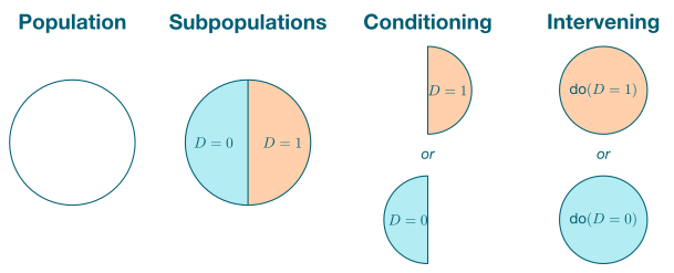
d-Separation lets us read independencies off a graph. But identification needs one more idea: a precise way to talk about intervening on a variable rather than merely observing it. The do-operator \(do(D = d)\) is that idea. It distinguishes between two distributions that look superficially alike but answer different questions:
- \(P(Y \mid D = d)\) is the observational distribution among units that happen to have \(D = d\).
- \(P(Y \mid do(D = d))\) is the interventional distribution we would see if every unit were forced to \(D = d\).
The first is what regression estimates from raw data. The second is what management actually wants to know. Whether they coincide is the entire question of causal identification.
Graph surgery. The do-operator has a concrete graphical meaning. To compute \(P(Y \mid do(D = d))\), take the original DAG \(G\) and delete every arrow into \(D\). The resulting mutilated graph \(G_{\overline{D}}\) has \(D\) with no parents — its value is no longer determined by its natural causes (including any confounders), but is instead set by the experimenter or decision-maker. The do-operator is then nothing more than ordinary conditioning in the mutilated graph:
\[P(Y \mid do(D = d)) \;=\; P_{G_{\overline{D}}}(Y \mid D = d).\]
A randomized experiment is the empirical realization of exactly this surgery: randomization severs every link from a unit’s covariates to its assigned treatment, so \(D\) in the experiment behaves like \(D\) in \(G_{\overline{D}}\).
The factorization swap. Why exactly are conditioning and intervention different? Compare the two derivations of \(P(Y \mid \cdot)\) for a DAG with confounder \(X \to D\), \(X \to Y\), \(D \to Y\):
| Step | Observational (\(D = d\)) | Interventional (\(do(D = d)\)) |
|---|---|---|
| Joint factorization | \(P(X)\,P(D \mid X)\,P(Y \mid D, X)\) | \(P(X)\,\cancel{P(D \mid X)}\,P(Y \mid D, X)\) |
| Distribution of \(X\) | \(P(X \mid D = d) = \dfrac{P(X)\,P(D = d \mid X)}{P(D = d)}\) | \(P(X \mid do(D = d)) = P(X)\) |
| Resulting formula | \(\sum_x P(Y \mid D = d, x)\,P(X = x \mid D = d)\) | \(\sum_x P(Y \mid D = d, x)\,P(X = x)\) |
Both averages share the same kernel \(P(Y \mid D = d, X = x)\); they differ only in the weight placed on each stratum \(x\). The observational formula uses the post-treatment weight \(P(X \mid D = d)\), which is contaminated by selection into \(D\); the interventional formula uses the natural weight \(P(X)\), which is what we would see without any selection. The two coincide if and only if \(X \perp\!\!\!\perp D\) — which is exactly the condition that fails when \(X\) is a confounder. The single-line difference between the two formulas is the entire mathematical content of “correlation \(\neq\) causation.”
Proof: the interventional formula via truncated factorization
Take a DAG with variables \(V_1, \ldots, V_n\) and Bayesian-network factorization
\[P(V_1, \ldots, V_n) = \prod_{i=1}^{n} P(V_i \mid \text{Pa}(V_i)).\]
Intervening on \(V_j\) via \(do(V_j = v_j)\) replaces the factor \(P(V_j \mid \text{Pa}(V_j))\) with the indicator \(\mathbb{1}\{V_j = v_j\}\) — equivalently, it deletes that factor from the product (since the remaining sum collapses to the single value \(v_j\)). The resulting truncated factorization is
\[P(V_1, \ldots, V_n \mid do(V_j = v_j)) = \prod_{i \neq j} P(V_i \mid \text{Pa}(V_i)) \quad \text{evaluated at } V_j = v_j.\]
For the simple confounder DAG \(X \to D\), \(X \to Y\), \(D \to Y\):
\[P(X, Y \mid do(D = d)) = P(X)\,P(Y \mid D = d, X).\]
Marginalizing \(X\) yields the interventional formula
\[P(Y \mid do(D = d)) = \sum_{x} P(Y \mid D = d, X = x)\,P(X = x).\]
This is the same formula one obtains from the potential-outcomes framework under conditional exchangeability \(Y(d) \perp\!\!\!\perp D \mid X\) — two languages for one assumption. Session 03’s backdoor criterion generalizes this construction to any DAG.
3.4 Coding Lab
3.4.1 Exercise 1: Building and Querying DAGs
Difficulty: Basic | Estimated time: 25 minutes
A marketing analytics team is trying to understand the drivers of customer lifetime value (CLV). Based on domain expertise, they believe the following causal structure holds:
- Marketing Budget (\(B\)) directly affects Ad Spending (\(A\)) and Brand Awareness (\(W\))
- Ad Spending (\(A\)) directly affects Customer Acquisition (\(C\))
- Brand Awareness (\(W\)) directly affects Customer Acquisition (\(C\)) and CLV (\(Y\))
- Customer Acquisition (\(C\)) directly affects CLV (\(Y\))
Tasks:
- Translate the verbal description into a DAG using code. Plot the DAG.
- Use software to check: Is \(A \perp\!\!\!\perp_G Y \mid \{W\}\)? Is \(A \perp\!\!\!\perp_G Y \mid \{C, W\}\)? Is \(B \perp\!\!\!\perp_G Y \mid \{A, W\}\)?
- List all implied conditional independencies of your DAG.
- Discuss: if one of the implied independencies were violated in data, what would that suggest about the DAG?
library(ggdag)
library(dagitty)

# (a) Define the DAG
dag <- dagify(
  # Fill in the edges based on the description
  # ___ ~ ___,
  # ___ ~ ___,
  coords = list(
    x = c(B = 0, A = 0, W = 1, C = 0.5, Y = 1),
    y = c(B = 1, A = 0, W = 1, C = 0, Y = 0)
  )
)

# Plot
dag |>
  ggplot(aes(x = x, y = y, xend = xend, yend = yend)) +
  geom_dag_point(colour = "#00C1D4", size = 20) +
  geom_dag_edges(edge_colour = "#005e73", edge_width = 0.8) +
  geom_dag_text(colour = "white", size = 4, fontface = "bold") +
  theme_dag()

# (b) Check d-separation
dseparated(dag, "A", "Y", c("W"))
dseparated(dag, "A", "Y", c("C", "W"))
dseparated(dag, "B", "Y", c("A", "W"))

# (c) List all implied conditional independencies
impliedConditionalIndependencies(dag)

# (d) Discussion: your answer here
from pgmpy.models import BayesianNetwork
from pgmpy.independencies import Independencies
# (a) Define the DAG
model = BayesianNetwork([
# Fill in edges as tuples: ("cause", "effect")
# ("___", "___"),
])
# (b) Check d-separation (note: is_dconnected is the opposite of dseparated!)
print("A ⊥ Y | {W}?", not model.is_dconnected("A", "Y", {"W"}))
print("A ⊥ Y | {C,W}?", not model.is_dconnected("A", "Y", {"C", "W"}))
print("B ⊥ Y | {A,W}?", not model.is_dconnected("B", "Y", {"A", "W"}))
# (c) List all implied conditional independencies
print(model.get_independencies())
# (d) Discussion: your answer here
TipShow solution
Show solution
library(ggdag)
library(dagitty)

# (a) Define the DAG
dag <- dagify(
  A ~ B,
  W ~ B,
  C ~ A + W,
  Y ~ W + C,
  coords = list(
    x = c(B = 0, A = 0, W = 1, C = 0.5, Y = 1),
    y = c(B = 1, A = 0, W = 1, C = 0, Y = 0)
  )
)

dag |>
  ggplot(aes(x = x, y = y, xend = xend, yend = yend)) +
  geom_dag_point(colour = "#00C1D4", size = 20) +
  geom_dag_edges(edge_colour = "#005e73", edge_width = 0.8) +
  geom_dag_text(colour = "white", size = 4, fontface = "bold") +
  theme_dag()
Show solution
# (b) d-Separation checks
cat("A ⊥ Y | {W}?", dseparated(dag, "A", "Y", c("W")), "\n")
A ⊥ Y | {W}? FALSE Show solution
cat("A ⊥ Y | {C,W}?", dseparated(dag, "A", "Y", c("C", "W")), "\n")A ⊥ Y | {C,W}? TRUE Show solution
cat("B ⊥ Y | {A,W}?", dseparated(dag, "B", "Y", c("A", "W")), "\n")B ⊥ Y | {A,W}? TRUE Show solution
# (c) Implied conditional independencies
impliedConditionalIndependencies(dag)
A _||_ W | B
A _||_ Y | C, W
B _||_ C | A, W
B _||_ Y | C, W
B _||_ Y | A, WAnswers:
- The d-separation results:
- \(A \perp\!\!\!\perp_G Y \mid \{W\}\): FALSE. Conditioning on \(W\) blocks the path through \(W\), but the path \(A \rightarrow C \rightarrow Y\) remains open.
- \(A \perp\!\!\!\perp_G Y \mid \{C, W\}\): TRUE. Both paths from \(A\) to \(Y\) are blocked: \(A \rightarrow C \rightarrow Y\) is blocked by \(C\) (chain), and \(A \leftarrow B \rightarrow W \rightarrow Y\) is blocked by \(W\) (fork).
- \(B \perp\!\!\!\perp_G Y \mid \{A, W\}\): TRUE. All paths from \(B\) pass through either \(A\) or \(W\), and both are conditioned on.
- If an implied conditional independence is violated in data (e.g., \(A\) and \(Y\) remain associated even after conditioning on \(\{C, W\}\)), this suggests the DAG is missing an edge. Perhaps \(A\) has a direct effect on \(Y\) not mediated by \(C\) or \(W\), or there is an unobserved common cause of \(A\) and \(Y\). This is the falsifiability property of DAGs — they generate testable predictions.
from pgmpy.models import BayesianNetwork

# (a) Define the DAG
model = BayesianNetwork([
    ("B", "A"),
    ("B", "W"),
    ("A", "C"),
    ("W", "C"),
    ("W", "Y"),
    ("C", "Y"),
])

# (b) d-Separation checks (pgmpy uses d-connected, so negate)
print("A ⊥ Y | {W}?", not model.is_dconnected("A", "Y", {"W"}))
print("A ⊥ Y | {C,W}?", not model.is_dconnected("A", "Y", {"C", "W"}))
print("B ⊥ Y | {A,W}?", not model.is_dconnected("B", "Y", {"A", "W"}))

# (c) Implied conditional independencies
print(model.get_independencies())
3.4.2 Exercise 2: d-Separation Challenge — a 10-node DAG
Difficulty: Challenge | Estimated time: 35 minutes
You are handed a complex causal graph from a colleague. Before running any analysis, you must verify which conditioning sets achieve d-separation between treatment \(D\) and outcome \(Y\). The DAG has 10 nodes:
- \(D\): treatment
- \(Y\): outcome
- \(W_1, W_2, W_3\): pre-treatment confounder chain (\(W_2 \rightarrow W_1 \rightarrow D\), \(W_2 \rightarrow W_3 \rightarrow Y\))
- \(M_1, M_2\): mediator chain (\(D \rightarrow M_1 \rightarrow M_2 \rightarrow Y\))
- \(X_1\): descendant of \(D\) (\(D \rightarrow X_1\))
- \(X_3\): descendant of \(Y\) (\(Y \rightarrow X_3\))
- \(X_2\): collider on the descendants (\(X_1 \rightarrow X_2 \leftarrow X_3\))
Tasks:
- Build the DAG in code and plot it. Layout coordinates are suggested below.
- For each of the six conditioning sets, predict by hand whether \(D \perp\!\!\!\perp_G Y\):
- \(\emptyset\)
- \(\{W_2\}\)
- \(\{W_2, M_1\}\)
- \(\{W_1, M_2\}\)
- \(\{W_1, M_2, X_2\}\)
- \(\{W_1, M_2, X_2, X_3\}\)
- Verify each prediction with software. Where you were wrong, identify the path you missed.
- Conditioning sets 5 and 6 differ only by adding \(X_3\). Explain what changes when \(X_3\) joins the conditioning set, and which structure (chain / fork / collider) is responsible.
library(ggdag)
library(dagitty)

# (a) Build the DAG
dag <- dagify(
  # Fill in the edges based on the description
  # ___ ~ ___,
  coords = list(
    x = c(D = 0, W1 = 1, W2 = 1.5, W3 = 2,
          M1 = 1, M2 = 2, Y = 3,
          X1 = 1, X2 = 1.5, X3 = 2),
    y = c(D = -1, W1 = 0, W2 = 0.5, W3 = 0,
          M1 = -1, M2 = -1, Y = -1,
          X1 = -2, X2 = -2.5, X3 = -2)
  )
)

# Plot
dag |>
  ggplot(aes(x = x, y = y, xend = xend, yend = yend)) +
  geom_dag_point(colour = "#00C1D4", size = 18) +
  geom_dag_edges(edge_colour = "#005e73", edge_width = 0.7) +
  geom_dag_text(colour = "white", size = 3.5, fontface = "bold") +
  theme_dag()

# (b) Your predictions for each conditioning set:
#  1. {}            : ___
#  2. {W2}          : ___
#  3. {W2, M1}      : ___
#  4. {W1, M2}      : ___
#  5. {W1, M2, X2}  : ___
#  6. {W1, M2, X2, X3} : ___

# (c) Verify with software
cat("1. {}:                  ", dseparated(dag, "D", "Y", c()),                         "\n")
cat("2. {W2}:                ", dseparated(dag, "D", "Y", c("W2")),                     "\n")
cat("3. {W2, M1}:            ", dseparated(dag, "D", "Y", c("W2","M1")),                "\n")
cat("4. {W1, M2}:            ", dseparated(dag, "D", "Y", c("W1","M2")),                "\n")
cat("5. {W1, M2, X2}:        ", dseparated(dag, "D", "Y", c("W1","M2","X2")),           "\n")
cat("6. {W1, M2, X2, X3}:    ", dseparated(dag, "D", "Y", c("W1","M2","X2","X3")),      "\n")

# (d) Explain the difference between (5) and (6) here.
from pgmpy.models import BayesianNetwork
# (a) Build the DAG (note: pgmpy uses tuples (cause, effect))
model = BayesianNetwork([
# Fill in edges as ("parent", "child")
# ("___", "___"),
])
# (b) Your predictions for each conditioning set go in comments
# (c) Verify (note: is_dconnected is the OPPOSITE of d-separated, so negate)
print("1. {}: ", not model.is_dconnected("D", "Y", set()))
print("2. {W2}: ", not model.is_dconnected("D", "Y", {"W2"}))
print("3. {W2, M1}: ", not model.is_dconnected("D", "Y", {"W2","M1"}))
print("4. {W1, M2}: ", not model.is_dconnected("D", "Y", {"W1","M2"}))
print("5. {W1, M2, X2}: ", not model.is_dconnected("D", "Y", {"W1","M2","X2"}))
print("6. {W1, M2, X2, X3}: ", not model.is_dconnected("D", "Y", {"W1","M2","X2","X3"}))
# (d) Explain the difference between (5) and (6) here.
TipShow solution
Show solution
library(ggdag)
library(dagitty)

# (a) Build the DAG
dag <- dagify(
  Y  ~ M2 + X3 + W3,
  W3 ~ W2,
  W1 ~ W2,
  D  ~ W1,
  M1 ~ D,
  M2 ~ M1,
  X1 ~ D,
  X3 ~ Y,
  X2 ~ X1 + X3,
  coords = list(
    x = c(D = 0, W1 = 1, W2 = 1.5, W3 = 2,
          M1 = 1, M2 = 2, Y = 3,
          X1 = 1, X2 = 1.5, X3 = 2),
    y = c(D = -1, W1 = 0, W2 = 0.5, W3 = 0,
          M1 = -1, M2 = -1, Y = -1,
          X1 = -2, X2 = -2.5, X3 = -2)
  )
)

dag |>
  ggplot(aes(x = x, y = y, xend = xend, yend = yend)) +
  geom_dag_point(colour = "#00C1D4", size = 18) +
  geom_dag_edges(edge_colour = "#005e73", edge_width = 0.7) +
  geom_dag_text(colour = "white", size = 3.5, fontface = "bold") +
  theme_dag()
Show solution
# (c) Verify all six conditioning sets
cat("1. {}:                  ", dseparated(dag, "D", "Y", c()),                         "\n")
1. {}: FALSE Show solution
cat("2. {W2}: ", dseparated(dag, "D", "Y", c("W2")), "\n")2. {W2}: FALSE Show solution
cat("3. {W2, M1}: ", dseparated(dag, "D", "Y", c("W2","M1")), "\n")3. {W2, M1}: TRUE Show solution
cat("4. {W1, M2}: ", dseparated(dag, "D", "Y", c("W1","M2")), "\n")4. {W1, M2}: TRUE Show solution
cat("5. {W1, M2, X2}: ", dseparated(dag, "D", "Y", c("W1","M2","X2")), "\n")5. {W1, M2, X2}: FALSE Show solution
cat("6. {W1, M2, X2, X3}: ", dseparated(dag, "D", "Y", c("W1","M2","X2","X3")), "\n")6. {W1, M2, X2, X3}: TRUE Answers:
There are three structural paths between \(D\) and \(Y\):
- P1 (causal mediator chain): \(D \rightarrow M_1 \rightarrow M_2 \rightarrow Y\)
- P2 (backdoor through pre-treatment fork): \(D \leftarrow W_1 \leftarrow W_2 \rightarrow W_3 \rightarrow Y\)
- P3 (descendants with collider \(X_2\)): \(D \rightarrow X_1 \rightarrow X_2 \leftarrow X_3 \leftarrow Y\)
Working set by set:
| # | Set | \(D \perp\!\!\!\perp_G Y\)? | Why |
|---|---|---|---|
| 1 | \(\emptyset\) | FALSE | P1 (chain) and P2 (fork) both open. P3 blocked by collider \(X_2\). |
| 2 | \(\{W_2\}\) | FALSE | P2 blocked by \(W_2\) (fork). P1 still open. |
| 3 | \(\{W_2, M_1\}\) | TRUE | P1 blocked by \(M_1\), P2 blocked by \(W_2\), P3 blocked (collider). |
| 4 | \(\{W_1, M_2\}\) | TRUE | P1 blocked by \(M_2\), P2 blocked by \(W_1\), P3 blocked. |
| 5 | \(\{W_1, M_2, X_2\}\) | FALSE | Same as (4) but conditioning on the collider \(X_2\) opens P3. |
| 6 | \(\{W_1, M_2, X_2, X_3\}\) | TRUE | P3 had been re-opened by \(X_2\); conditioning on \(X_3\) (a parent of the collider, on the path to \(Y\)) re-blocks it as a chain \(D \rightarrow X_1 \rightarrow X_2\) no longer connects to \(Y\) once \(X_3\) is held fixed. |
- The pivotal change between (5) and (6) is the role of the collider \(X_2\). Adding \(X_2\) to the conditioning set in (5) opens path P3 — the classic collider trap. Adding \(X_3\) in (6) re-closes the path because \(X_3\) is the parent of \(X_2\) on the side that connects to \(Y\); with \(X_3\) fixed, the only way information about \(Y\) could leak through \(X_2\) is severed. This is a clean illustration of why “control for everything” fails: variable \(X_2\) alone is harmful, but \(X_2\) together with \(X_3\) is harmless.
from pgmpy.models import BayesianNetwork

model = BayesianNetwork([
    ("M2", "Y"), ("X3", "Y"), ("W3", "Y"),
    ("W2", "W3"), ("W2", "W1"),
    ("W1", "D"),
    ("D", "M1"), ("M1", "M2"),
    ("D", "X1"), ("Y", "X3"),
    ("X1", "X2"), ("X3", "X2"),
])

print("1. {}:                  ", not model.is_dconnected("D", "Y", set()))
print("2. {W2}:                ", not model.is_dconnected("D", "Y", {"W2"}))
print("3. {W2, M1}:            ", not model.is_dconnected("D", "Y", {"W2","M1"}))
print("4. {W1, M2}:            ", not model.is_dconnected("D", "Y", {"W1","M2"}))
print("5. {W1, M2, X2}:        ", not model.is_dconnected("D", "Y", {"W1","M2","X2"}))
print("6. {W1, M2, X2, X3}:    ", not model.is_dconnected("D", "Y", {"W1","M2","X2","X3"}))
3.5 References & Resources
3.5.1 Academic Literature
- Pearl, J. (2009). Causality: Models, Reasoning, and Inference. 2nd ed. Cambridge University Press. — The foundational reference for DAGs and the do-operator. Chapters 1 (probabilities and graphs) and parts of Chapter 3 (interventions and graph surgery) are most relevant here; the identification chapters of Pearl are taken up in Session 03.
- Pearl, J., Glymour, M. & Jewell, N. P. (2016). Causal Inference in Statistics: A Primer. Wiley. — The accessible companion. Chapters 1–3 cover DAG semantics, d-separation, and the do-operator at the level of this session.
- Elwert, F. (2013). Graphical Causal Models. In S. L. Morgan (Ed.), Handbook of Causal Analysis for Social Research. Springer, 245–273. — Concise exposition of DAGs, building blocks, and d-separation aimed at social-science readers.
- Hernán, M. A. & Robins, J. M. (2020). Causal Inference: What If. Chapman & Hall/CRC. — Chapter 6 introduces graphs and confounding from an epidemiological angle; pairs well with this session’s chains/forks/colliders pass.
- Neal, B. (2020). Introduction to Causal Inference. — Chapter 3 (DAGs and d-separation) and Chapter 4 (the do-operator and graph surgery) are the closest free-text mirror of this session. The “conditioning vs. intervention” figure used on the slides is adapted from his Chapter 4.
- Cunningham, S. (2021). Causal Inference: The Mixtape. Yale University Press. — Chapter 3’s DAG primer with economics applications and intuitions for the building blocks.
- Hünermund, P. & Bareinboim, E. (2023). Causal Inference and Data Fusion in Econometrics. The Econometrics Journal, 26(1), 1–34. — Bridges the DAG and potential-outcomes frameworks; the “PO–DAG bridge” we sketch in the do-Operator section is a small piece of their argument.
- Imbens, G. W. (2020). Potential Outcome and Directed Acyclic Graph Approaches to Causality. Journal of Economic Literature, 58(4), 1129–1179. — Balanced comparison of the PO and DAG frameworks for economists.
3.5.2 Practitioner Resources
- DAGitty — Interactive web tool for drawing DAGs, checking d-separation, and finding adjustment sets. Essential companion for this session.
- Tennant, P. W. G. et al. (2021). Use of Directed Acyclic Graphs (DAGs) to Identify Confounders in Applied Health Research. International Journal of Epidemiology, 50(2), 620–632. — Practical tutorial on using DAGs for covariate selection in applied research.
- Causal Inference: Three Frameworks (2025). — Recent comparison of SCM, potential outcomes, and decision-theoretic frameworks.
- Textor, J., van der Zander, B., Gilthorpe, M. S., Liśkiewicz, M. & Ellison, G. T. H. (2016). Robust Causal Inference Using Directed Acyclic Graphs: The R Package
dagitty. International Journal of Epidemiology, 45(6), 1887–1894. — ThedagittyR package paper with usage examples.