17 Session: Counterfactual Imputation

17.1 Lecture Slides

Open slides in new tab | Download as PDF

17.2 Overview

S11 closed on a quiet image — a synthetic-control weight vector is just a row of instructions for rebuilding one unit’s outcome from the others, and stacking such rows is a matrix operation. This final session cashes that image into the unifying claim of the whole course. Look at the BeanBuzz store panel — 233 stores × 104 weeks, balanced, with 158 stores eventually launching the loyalty app and 75 never doing so — as a grid with a blanked-out region: the 5,606 treated store-weeks whose untreated potential outcome $Y(0)$ we can never observe. Every average treatment effect anyone reported in Part V is observed minus imputed over that grey block, so the causal question is literally a missing-data problem: predict the grey cells from the white ones. The organizing move is that every panel estimator since Part III solves the same penalized least-squares problem — fit the observed cells, pay a penalty for the reconstruction — and differs only in the penalty, which is the structural assumption on the cells you can never check (Athey et al. 2021; Arkhangelsky and Imbens 2024).

The three estimators the session formalizes are nested rungs of one dial: fect’s FEct (method="fe", additive, the dial at $r=0$), IFEct (method="ife", a rank-$r$ factor, hard-impute), and matrix completion (method="mc", a nuclear-norm penalty, soft-impute). FEct is not a different animal — it is IFEct with the dial turned to zero, so ife and mc are extensions of the fe imputation estimator, not competitors (Liu, Wang, and Xu 2024). The anchor that grounds the dial is an exact identity: the Borusyak-Jaravel-Spiess imputation estimator (didimputation), fect’s FEct, and a hand-rolled “fit FE on the white cells, predict the grey ones” recipe all return +4.23% to the digit (max abs difference $< 10^{-5}$) — DiD under two-way FE is not like an imputation, it is one, and it is the dial at $r=0$.

That honest +4.23% sits below the true +4.93%, not from selection but from blindness: additivity cannot represent a latent wave that stores ride by different amounts. Turn the dial up and a low-rank model sees it: IFEct picks $r=1$ by cross-validation and climbs to +4.76%, its estimated factor matching the dominant data-generating wave — a slow regional-economy cycle — at correlation 0.999. The honest counterweight the session refuses to soft-pedal is that matrix completion under-recovers (+4.31%): its nuclear-norm penalty shrank the very factor it needed — more flexible is not more right. Then the truth line is taken away. From the sensitivity act onward the rank is fixed at the CV pick ($r=1$) and every claim must be derivable from what fect prints on your own screen — because that is the only situation you will ever actually be in. The session stress-tests the answer against parallel-trends violations and finds there is no verdict, only a price: fect computes three pre-trend tests against three different nulls and shows only two by default (the hidden one is the only one that certifies), and one argument you never passed (proportion) flips the panel into certifying its own pre-trend. The placebo is then demoted from a gate to a ruler — it fires and passes on the same figure, so significance is not size — and its largest blanked-window step (0.240 pp) becomes the unit every bound is denominated in. Relative magnitudes exposes three hidden dials: $\bar M = 0$ turns out to be a frozen violation rather than none (the arithmetic $3.13 - 0.88 = 2.25$ proves it, and it is the opposite of what $\bar M=0$ meant in S10, where an omitted base period made it exact parallel trends); the sweep’s upper edge is censored at HonestDiD’s search-grid ceiling (13 of 21 bounds pinned, the warning swallowed); and the grid resolution itself moves the answer ($\bar M^{*} = 0.50$ coarse, 0.46 refined). The breakdown value is therefore reported as a pair — 0.46, which on this fit is 0.11 pp of drift per week — because a model that fits its pre-window better cuts a shorter ruler and earns a bigger $\bar M^{*}$ for free.

The session then opens up the heterogeneity the +4.8% average hides — and the first thing it does is refuse to read it, twice, on the same fit. Read the cells: one store-week in five reads negative — but box the pre-launch window, where nothing happened, and 48% of cells read negative too. The null value of that statistic is 50, not 0 — a normal-equations identity (treatment is absorbing, so each store’s unit FE is fitted on exactly its own pre-cells) that four imputers of wildly different quality all reproduce, and that holds whatever the true pre-effect is. So aggregate instead — and ask when: the calendar-week ATT climbs +1.25% → +5.80%, a swing as large as the ATT itself, and there is no calendar in it. It is the tenure ramp sampled through a staggered rollout — a reconstruction carrying no calendar term at all lands inside the estimate’s own CI in 48 of 52 weeks, and the dips fall exactly on the go-live waves. Neither number is wrong; both readings are. Then fect refuses the moderator you want (urban_share is unit-invariant) while cheerfully drawing a curve for one your treatment moved — the API’s constraint selects for bad controls — and the honest route, group=, delivers a real 5.75-point spread that the session immediately catches on composition (36% of it is rollout timing on a ramping effect) and then audits with a per-group placebo: the one group a board would deprioritise is the one group whose number it cannot use. It closes on the completed assumption ledger — the A5 rubric — and the discipline carried verbatim from S10 and S11: a point estimate without a defensible assumption and a band is not a finding.

Learning objectives. By the end of this session you will be able to:

Name the move every panel estimator makes since Part III — impute the blanked $Y(0)$ block of treated cells — and point to the greyed BeanBuzz matrix (5,606 treated cells) as the shared object, distinguishing prediction at the design layer (causation $\neq$ prediction) from prediction at the estimation layer (causation is prediction, once identified).
Write the generalized objective $\min_L \sum_{\mathcal{O}}(Y-L)^2 + \lambda\cdot\text{penalty}(L)$ and place FEct / IFEct / MC on it as one nested dial — additive ($r=0$), hard-impute (rank $r$), soft-impute (nuclear norm) — stating each one’s assumption as a business sentence.
Prove that DiD under two-way FE is imputation: show FEct = BJS = a hand-rolled FE-imputation = +4.23% to the digit, in R and Python, and recognize it as the dial at $r=0$.
Explain and exhibit why a low-rank factor model (IFEct $r=1$) recovers the omitted latent factor two-way FE is blind to (+4.23% → +4.76% → true +4.93%) — and why “more flexible” $\neq$ “more right” (matrix completion +4.31%, the under-recovery lesson).
Stress-test a factor model with no answer key: read all three pre-trend tests fect computes against their three different nulls (and ask for the hidden one that actually certifies), recognise that the verdict is set by defaults you never chose (the window, the band, the grid), turn the placebo from a gate into a ruler (0.240 pp — a step, not a level), and report a relative-magnitudes breakdown as a pair ($\bar M^{*} = 0.46$ = 0.11 pp of drift per week) — knowing that $\bar M = 0$ is a frozen violation rather than none, that fect_sens’s upper bounds are censored until checked against $20\times\text{SE}$, and that a bare $\bar M^{*}$ is never comparable across models.
Know what an effect matrix will and will not tell you: refuse to read a cell (the null value of “% of store-weeks reading negative” is 50, not 0 — a normal-equations identity that holds whatever the true pre-effect is), diagnose why the API’s own constraint selects for bad controls, and reach heterogeneity the honest way — a group= split (+7.3% / +4.6% / +1.6%) that you then catch on composition (36% of it is rollout timing) and audit with a per-group placebo that can convict but never acquit.
Decide: run a method bake-off and write a 4-sentence board memo that picks one estimator by assumption credibility, reports a band, and matches each of A5’s two estimands to its lens — the single flagship to synthetic control, the staggered pilot portfolio to the many-unit DiD/imputation pipeline.

17.3 Lecture Notes

17.3.1 Every causal number fills a blank you never saw

17.3.1.1 The grey cells

Hold the spreadsheet image from S10 and S11 one final time, now made literal (Figure 17.1). The BeanBuzz store panel is a grid: 233 stores down the rows, 104 weeks across the columns, and the data themselves are balanced — every store is observed in every week, with no mechanical gaps. The only missingness is causal. Of the 233 stores, 158 eventually launch the loyalty app (the treated) and 75 never do (the clean control pool — the white cells we can lean on throughout). For each treated store, every week after its own launch is a treated cell; counting them gives exactly 5,606 treated store-weeks. In each of those 5,606 cells we observe $Y(1)$ — the store’s revenue with the app — but the average treatment effect needs $Y(0)$, what that same store would have earned without it, and $Y(0)$ is by definition never observed for a treated cell. That is the greyed-out staircase. It is ragged, not rectangular, because stores launched in waves (the staggered adoption of S10), so each treated store’s blank begins at a different week.

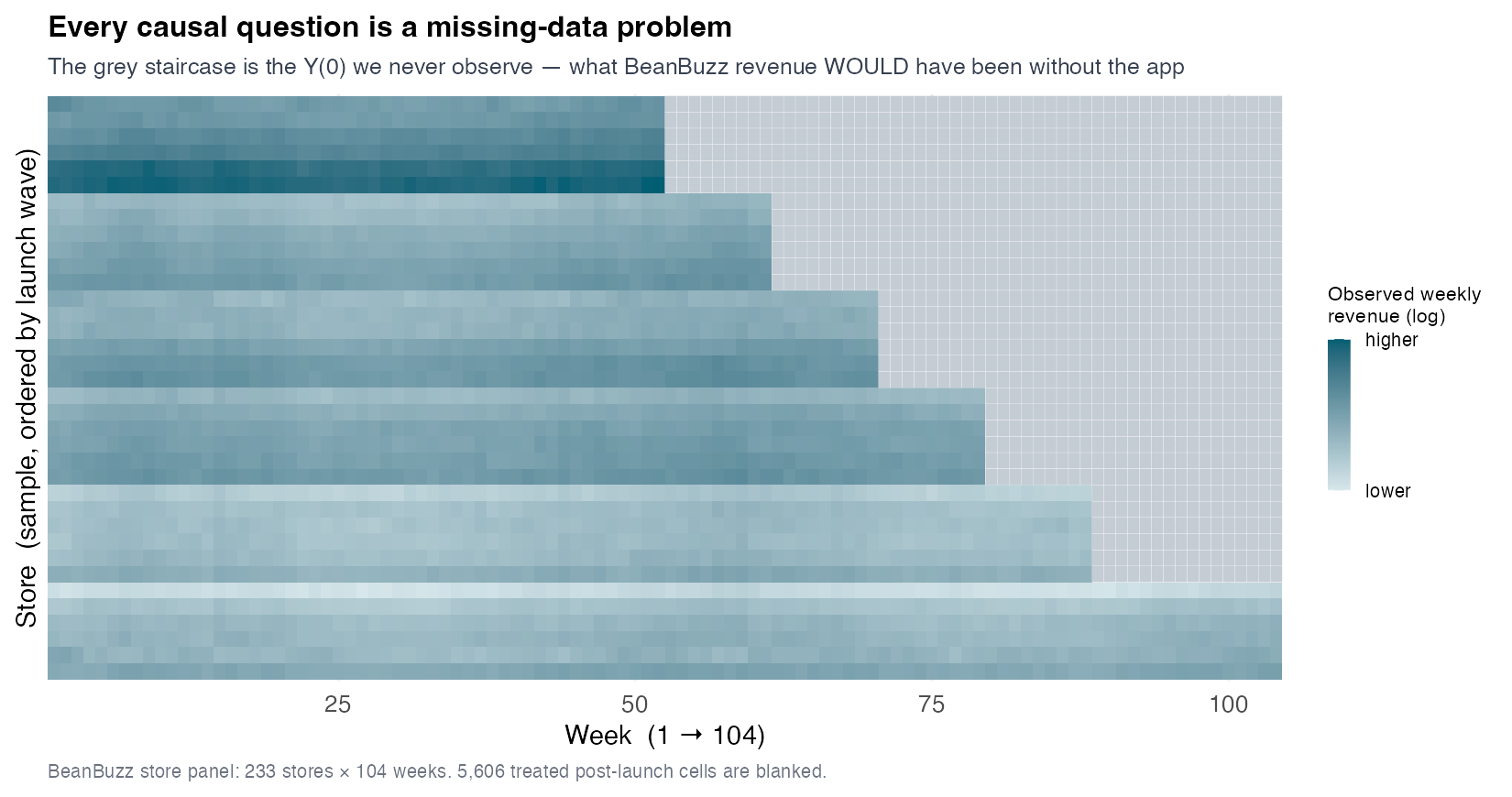
Figure 17.1: A units-by-time grid of 233 BeanBuzz stores down the rows and 104 weeks across the columns. Observed cells are shaded; a large ragged block of treated-store cells after each store’s launch week is greyed out and blank, marking the unobserved untreated potential outcome $Y(0)$. The blanked region forms a staircase because stores launched in different weeks (staggered adoption). The white cells — the 75 never-treated stores plus every treated store’s pre-launch history — are the training data; the grey staircase is the test set.

Every ATT reported across Part V is the gap between a number you saw (observed treated revenue) and a number you imputed (predicted $Y(0)$), averaged over those 5,606 grey cells. The board only ever sees the headline; the entire methodological content of the part lives in how the grey was filled. This reframing — every causal number on a panel is a prediction of an unobserved cell — is the conceptual unlock for the session.

17.3.1.2 Prediction is not causation — but causation is a prediction problem

Students carry a refrain from week one: correlation predicts; it does not identify a cause (Athey and Imbens 2017). A black-box model that forecasts revenue beautifully tells you nothing about what the app did, because it confounds treatment with everything correlated with it. That warning is correct and stays correct — but it operates at the identification layer: which comparisons are valid, which cells count as clean controls, what assumption licenses the counterfactual. Once that design layer is settled — and Part V settled it, via parallel trends, donor hulls, or factor structure — what remains is a pure prediction task: use the observed cells to forecast the unobserved $Y(0)$ cells, then subtract. Both slogans are true, at different layers:

Causation $\neq$ prediction at the design layer — a good predictor of $Y$ need not give a valid counterfactual (Ferman’s S11 lesson: a flawless pre-fit can still be a biased counterfactual).
Causation $=$ prediction at the estimation layer — with the design fixed, the ATT is the mean of observed $-$ predicted $Y(0)$ over the grey block.

Athey and Imbens make this precise: modern causal panel methods are imputation estimators (Athey et al. 2021). This is the hinge that lets the rest of the session talk about “filling cells” without abandoning causal rigor — the rigor lives in the design; the arithmetic lives in the prediction.

17.3.1.3 Four methods, one secret job

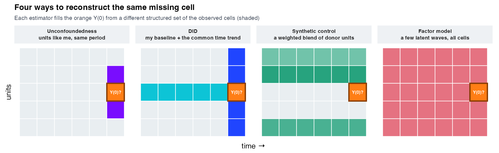
Every panel tool met since Part III does the same thing — predict the grey block — under a different cover story (Figure 17.2):

Unconfoundedness / matching (Part III): impute $Y(0)$ from units that look like me on covariates.
DiD / two-way FE (S10): impute $Y(0)$ from a common time trend plus my own baseline.
Synthetic control (S11): impute $Y(0)$ from a bespoke donor blend matched on my past.
Interactive-FE / matrix completion (today): impute $Y(0)$ from a few latent factors everyone loads on.

Four chapters, one job. The headline climbs as the cover story gets richer and absorbs more structure: from the additive family near +4.2% toward the true +4.9%. That climb is the whole empirical narrative of the session; everything after this point is detail on why and how it happens.

Figure 17.2: Four small copies of the same units-by-time panel side by side, each with the identical grey treated block. In each copy, arrows reach from a different set of observed white cells into one grey target cell: covariate-similar units, a column-wise time trend, a weighted donor blend, and a low-rank factor reconstruction. The target blank is the same in all four; only the borrowing rule changes. Recall S11: a weight vector is just a *row*, and stacking such rows is a matrix operation.

17.3.2 One objective, one regularizer dial

17.3.2.1 The penalized-imputation objective

Make the unification formal. Write the panel of untreated potential outcomes as a units-by-time matrix $L$, of which we observe only the entries on the white cells (the set $\mathcal{O}$ of untreated store-weeks). Imputing the grey block means reconstructing the missing entries of $L$ from the observed ones. Every method in Figure 17.2 solves a version of the same penalized least-squares problem:

\[\min_{L}\ \sum_{(i,t)\in\mathcal{O}}\big(Y_{it} - L_{it}\big)^2 \;+\; \lambda\,\cdot\,\text{penalty}(L), \tag{17.1}\]

Read $L_{it}$ as the reconstructed untreated outcome $Y_{it}(0)$: on the white cells it is the fitted value the first term pins to the data, and on the grey treated cells it is the imputed counterfactual — the ATT averages the treated cells’ observed $Y_{it}-L_{it}$ over the grey block. The penalty is the only thing that changes (Athey et al. 2021; Arkhangelsky and Imbens 2024). The penalty is the structural assumption you impose on the grey cells you can never check — covariate balance, additivity, convex sparsity, or low rank. Choose the penalty and you have chosen your causal method; the unification is not a metaphor but a single objective with a swappable regularizer.

Table 17.1: The same imputation objective (Equation 17.1), four regularizers.

Method	What it borrows from	The regularizer encodes	Plain-English assumption
Unconfoundedness / matching	Units like me on covariates	Balance on measured $X$	“Given what I measured, treatment is as-good-as-random.”
DiD / TWFE	A common time trend + my baseline	$L_{it}=\alpha_i+\lambda_t$ (additive)	“Absent treatment, I’d have moved parallel to the controls.”
Synthetic control	A bespoke donor blend matched on my past	$L$-rows are convex blends of donor rows (sparse simplex)	“A weighted blend of donors tracks me before treatment.”
Interactive-FE / matrix completion	A few latent factors everyone loads on	$L=\alpha_i+\lambda_t+\sum_r L_{ir}F_{rt}$ (low rank)	“The panel is driven by a handful of shared shocks.”

Read each row of Table 17.1 as a borrowing rule plus the assumption that licenses it. Unconfoundedness regularizes toward covariate balance — right when covariates are rich but no panel time-structure can be exploited. DiD regularizes toward strict additivity ($\alpha_i+\lambda_t$) — right with many units and plausibly parallel pre-trends. Synthetic control regularizes the rows toward convex, sparse blends of donor rows — right for one or a few treated units with a clean donor pool. Interactive-FE and matrix completion regularize toward low rank — the panel is governed by a small number of latent shared shocks (a seasonality wave, a business cycle), and stores load on them by different amounts. The manager’s takeaway: you are always choosing an assumption about the cells, never just “a method.” Squared loss targets the mean $Y(0)$, so this is specifically the outcome-model / imputation move; where it sits among the other panel families — weighting (synthetic control / SDID, S11), doubly-robust (DR-DiD / DML, S10), distributional (Changes-in-Changes / quantile effects) — and the strict-exogeneity gate beneath all of them are laid out at the close, in the completed assumption ledger.

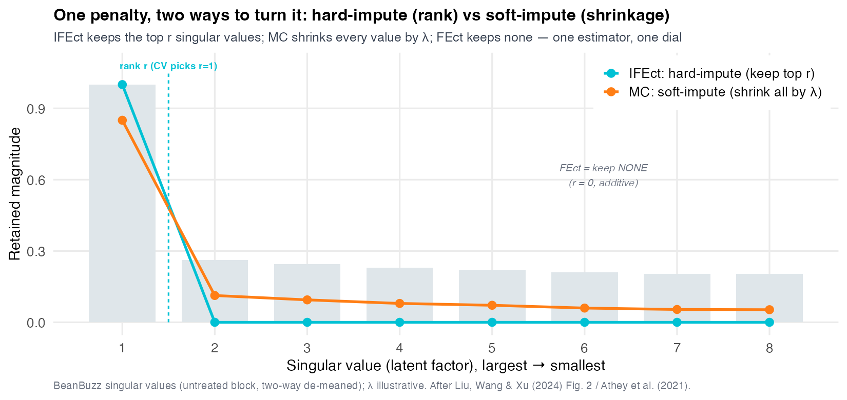
17.3.2.2 The penalty is a dial: FEct, IFEct and MC are one estimator

The three estimators are not a menu — they are one estimator at three settings of a single dial (Figure 17.3), and fect exposes them as one function call. Decompose the untreated panel; its singular values are the latent factors ordered by strength. FEct (method="fe") keeps none of them beyond the additive means — the dial at $r=0$. IFEct (method="ife") hard-imputes: keep the top $r$ singular values in full, drop the rest (a best-subset step). Matrix completion (method="mc") soft-imputes: shrink every singular value toward zero by $\lambda$ (an $L_1$/nuclear-norm penalty). The nesting is exact and load-bearing: FEct is IFEct at $r=0$, and MC collapses back to FEct once $\lambda$ exceeds the largest singular value (Liu, Wang, and Xu 2024). So ife and mc are extensions of the fe imputation estimator, not rivals — hard-impute keeps a few factors whole, soft-impute keeps all of them smaller, and both reduce to additivity at the bottom of the dial.

Figure 17.3: Retained magnitude of each singular value: the raw values as grey bars; the IFEct hard-impute path keeps the top r in full and drops the rest to zero (a step); the MC soft-impute path shrinks every value by lambda; FEct keeps none. One objective, one dial, two ways to turn it.

17.3.2.3 The regularizer is the assumption

Here is the uncomfortable truth the one-optimization view exposes. On the observed white cells, every method can be made to fit well — that is what fitting does. The methods only diverge on the grey cells, the ones you can never verify against ground truth. And on those cells, the entire difference between +4.2% and +4.9% is the regularizer’s assumption: additivity says the grey cells follow parallel trends; low rank says they follow a factor; convex sparsity says they follow a donor blend. The assumption, not the data, fills the blank.

Pick the assumption, not the p-value

The only honest basis for choosing a method is which assumption you can defend in this business context — is parallel trends plausible here, or is there obviously a latent wave (a regional cycle, a season) units ride by different amounts? — not which estimate has the prettiest standard error or the most convenient magnitude. This is the same discipline as Part IV’s “pick the identification strategy, not the significant coefficient,” and it is the through-line of the course’s final third: a method’s credibility is the credibility of its assumption on the cells you will never see. A point estimate without a defensible assumption behind it is not a finding. This is the sentence A5 is testing.

17.3.3 DiD is imputation — proven to the digit

17.3.3.1 The Borusyak recipe, re-named

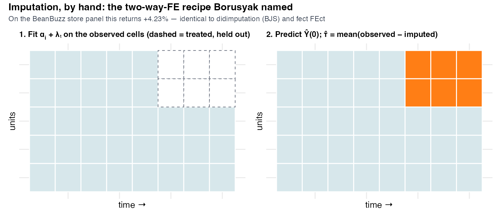
S10 introduced the imputation estimator of Borusyak, Jaravel and Spiess (BJS) as one robust DiD method among several — but its name already gives the game away: it is an imputation (Borusyak, Jaravel, and Spiess 2024). The three-step recipe is the formal version of everything Section 17.3.1 said in pictures, and it is exactly “fill the grey from the white”:

Fit unit and time fixed effects on the untreated (white) cells only — the 75 never-treated stores across all weeks, plus every treated store’s pre-launch history — so no treated outcome contaminates the $Y(0)$ model.
Predict each treated (grey) cell’s $Y(0)$ from those fitted effects: $\widehat{Y}_{it}(0)=\hat\alpha_i+\hat\lambda_t$.
Average observed $-$ imputed over the grey block: $\widehat{\text{ATT}} = \frac{1}{5606}\sum_{(i,t)\,\text{treated}}\big(Y_{it}-\widehat{Y}_{it}(0)\big)$.

The restriction in step 1 — fit only where app_live == 0 — is precisely what makes the prediction a clean counterfactual rather than a tautology (Figure 17.4). There is nothing inside the black box but a fixed-effects regression and a subtraction.

Figure 17.4: A schematic of the hand-rolled imputation. The left panel shows the panel with only the untreated white cells highlighted, labelled “fit two-way fixed effects here.” A central arrow labelled “predict” points to the right panel, where the previously grey treated cells are now filled with imputed $Y(0)$ values. Below, the observed-minus-imputed difference over the treated block is averaged to a single number, +4.23%.

17.3.3.2 Three computations, one number

This is the anchor of the session. Three computations that look completely different — the BJS imputation estimator from a published package (didimputation), the FEct (fixed-effects counterfactual) estimator from Liu-Wang-Xu’s fect package with method="fe", and the hand-rolled feols-plus-predict from the recipe above — all land on +4.23%, with a maximum absolute difference below $10^{-5}$ (Figure 17.5).

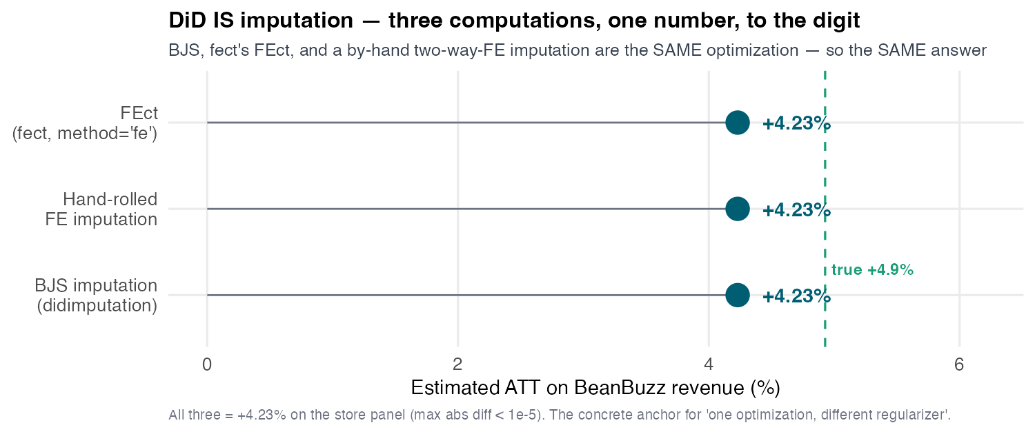
Figure 17.5: Three horizontal markers stacked on a common axis, all landing on exactly the same point at +4.23%. The top marker is labelled “BJS imputation,” the middle “fect FEct,” the bottom “hand-rolled two-way-FE imputation.” A bracket annotates that the maximum absolute difference between the three is less than $10^{-5}$. Not three methods that agree closely — one estimator written three ways.

This is not three methods that happen to agree closely; it is one estimator written three ways, and the tiny residual is floating-point noise, not statistical disagreement. The phrase “to the digit” is earned here, because unlike a confidence interval this identity is genuinely deterministic — restricted two-way-FE imputation is a fixed linear operation, so any correct implementation must return the same number. The conceptual payoff cashes the whole act: difference-in-differences under two-way fixed effects does not merely resemble an imputation of the missing block — it is one, exactly. The abstract claim from Section 17.3.2, “DiD is one regularizer on the imputation problem,” is now a proven equality you can run in both R and Python (Lab 1, the graded bilingual anchor).

17.3.3.3 But the honest number is still too low

The hand-rolled, identity-confirmed imputation is honest in every way students have been trained to check: it fits $Y(0)$ on uncontaminated untreated cells, it ignores no selection, it has no forbidden comparisons. And yet it sits at +4.23%, clearly below the oracle truth of +4.93%. This is not a selection artifact like the naive +16.3%. It is structural blindness.

What the additive model cannot represent

Two-way FE says $Y(0)=\alpha_i+\lambda_t$ — strictly additive, separable. That functional form literally cannot represent an interaction: a latent factor that moves over time and that different stores load on by different amounts. In BeanBuzz the data-generating process carries two such waves. The dominant one is a slow regional-economy cycle: whole regions boom and slump together, and regions differ sharply in how hard they ride it (its loading is region-level — $R^2 = 0.97$ on region). The fainter one is a coffee-seasonality wave: cold months lift hot-drink demand everywhere, but the common time effect $\lambda_t$ already absorbs the average lift, so seasonality survives only as the differential — urban, footfall-driven stores ride it harder than roadside drive-throughs — and that differential is roughly 6–8× smaller than the regional spread. Call the dominant regional wave $F_1$ and the fainter seasonality wave $F_2$ — that is the order the SVD returns them in, and we will keep it throughout. Unable to express store-specific exposure to a time-varying factor, the additive model effectively averages both waves into the common time effect and common store effect, and the residual store-time interaction leaks into the estimate as downward bias. An honest additive imputation can still be a blind one — honesty about contamination is necessary, not sufficient.

17.3.4 The factor DiD cannot see

17.3.4.1 Additive effects cannot bend; factors can

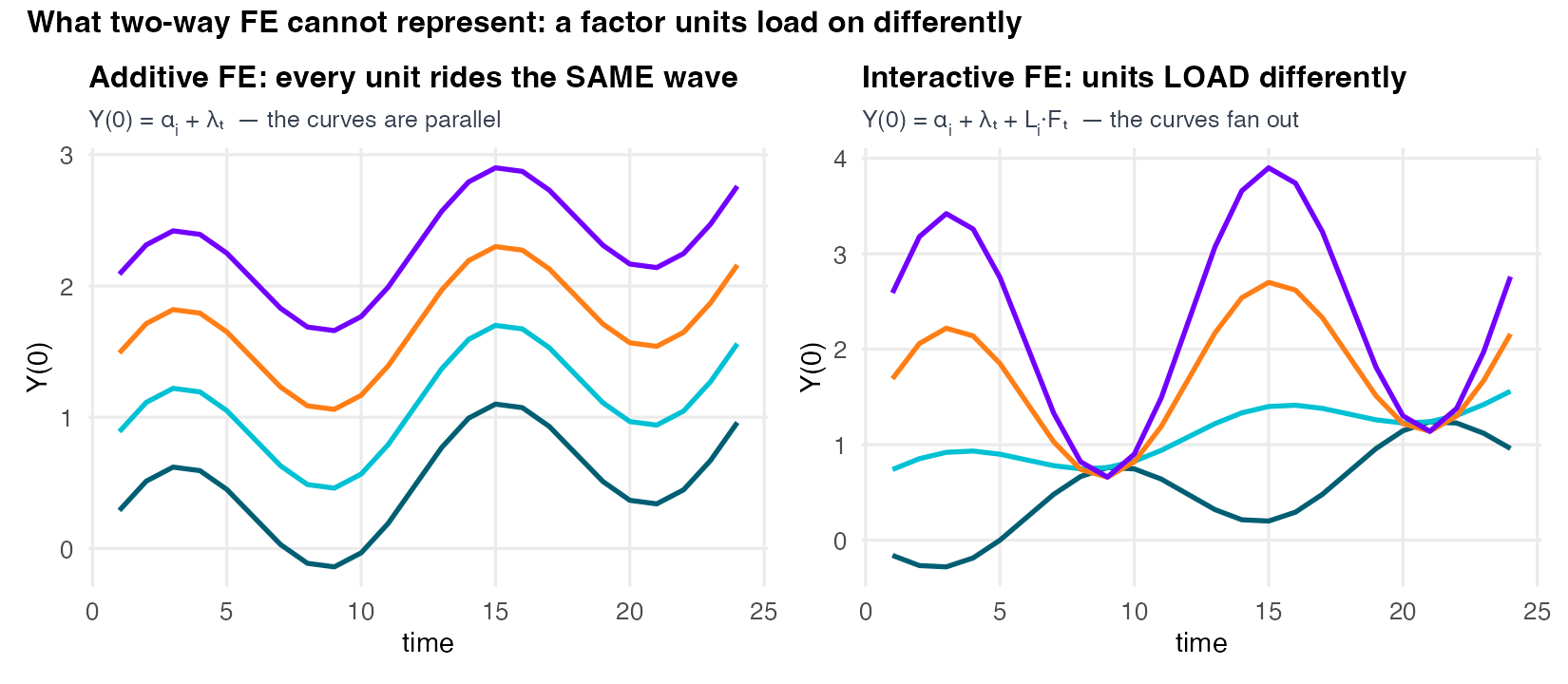
Make the functional-form difference visual (Figure 17.6). In the additive two-way-FE world, every store’s $Y(0)$ is its own level $\alpha_i$ plus a common time wiggle $\lambda_t$, so all paths are vertical shifts of the same curve — they stay strictly parallel, never crossing, never spreading. That parallelism is the parallel-trends assumption, drawn. The interactive-fixed-effects world adds one term:

\[\underbrace{Y_{it}(0)=\alpha_i+\lambda_t}_{\text{additive (DiD)}} \qquad\longrightarrow\qquad \underbrace{Y_{it}(0)=\alpha_i+\lambda_t+\textstyle\sum_{r=1}^{R} L_{ir}F_{rt}}_{\text{interactive FE / low rank}}. \tag{17.2}\]

The new term $L_{ir}F_{rt}$ is a store-specific loading $L_{ir}$ on a shared time-varying factor $F_{rt}$ (Liu, Wang, and Xu 2024; Xu 2017). Now stores fan: a store with a high loading on the shared wave swings more when that wave peaks, a low-loading store swings less, so the paths spread, reconverge, and can cross. The additive model cannot draw the right-hand picture no matter how you fit it — the $L_{ir}F_{rt}$ term is simply absent from its vocabulary. That is the precise sense in which DiD is “blind” to $L_{ir}F_{rt}$: the bias is not in the estimation, it is in the model class. The fix is not better fitting but a richer model — and crucially low rank means few factors: here a single factor ($R=1$) suffices, so this is one bend the additive model could not make, not a licence for arbitrary flexibility.

Figure 17.6: Two small multiples. On the left, additive two-way fixed effects: several store $Y(0)$ paths over time that stay strictly parallel, all rising and falling together by the same time effect. On the right, an interactive factor model: the same stores fan apart and reconverge as each loads by a different amount on a shared wavy factor, so the paths cross and spread rather than staying parallel.

17.3.4.2 One API, three regularizers

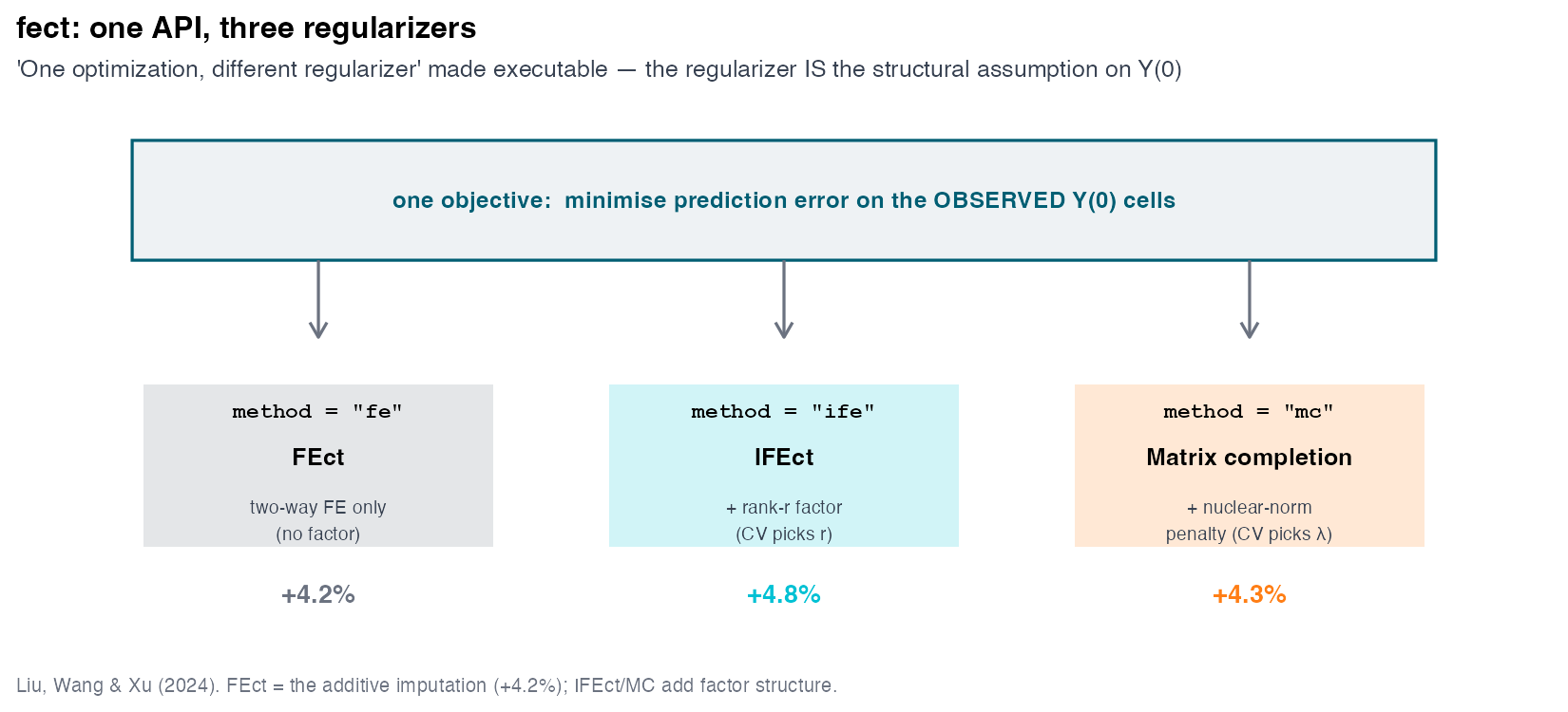
The unification is not merely conceptual — it is literally one function call with a switch, the most concrete possible proof of “one optimization, different regularizers.” Liu, Wang and Xu’s fect package exposes exactly the structure of Table 17.1 (Figure 17.7): hand it the same panel and toggle the method argument (Liu, Wang, and Xu 2024).

method = "fe" — additive two-way-FE imputation (the FEct that equalled BJS and the hand-roll to the digit, +4.23%).
method = "ife" — interactive fixed effects: adds the low-rank factor term, estimates loadings, recovers the latent wave the additive model missed.
method = "mc" — matrix completion: imputes the block under a nuclear-norm penalty (the nuclear norm is the sum of the matrix’s singular values; shrinking it drives those values toward zero, which is what encourages a low-rank fit) rather than fixing the factor count.

Three estimators, one API, three regularizers — additive, explicit low-rank factor, nuclear-norm shrinkage. The choice of causal method has collapsed into the choice of one string argument, because underneath they are the same imputation with different structure imposed.

Figure 17.7: A single function-call diagram. One fect call sits in the centre with a method argument that branches three ways: method equals fe to two-way fixed-effects imputation, method equals ife to interactive fixed effects, method equals mc to matrix completion. All three feed the same panel in and return an imputed $Y(0)$ block, differing only in the regularizer label beneath each branch: additive, low-rank factor, nuclear-norm.

17.3.4.3 Cross-validation picks one factor — and it is the regional wave

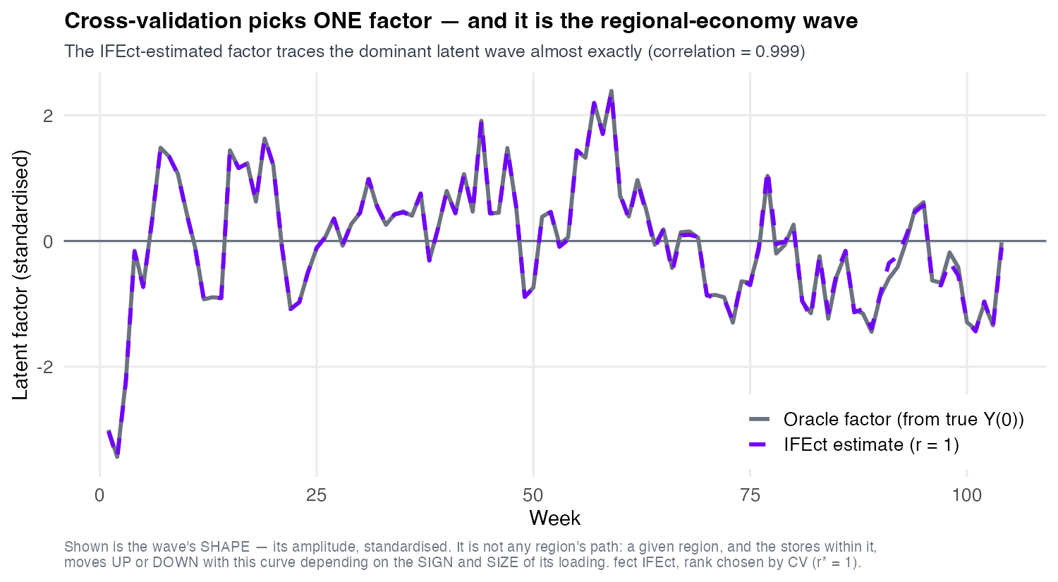
fect’s interactive-FE estimator does not need to be told how many factors there are; it selects the rank by cross-validation, hiding a block of observed pre-treatment weeks, forecasting them forward, and keeping the simplest rank whose held-out error is within one standard error of the best (fect’s default cv.rule = "1se"). On BeanBuzz it picks $r=1$ — a single factor — matching the dominant data-generating wave (the world carries two latent waves; CV bought a factor for the big one and, honestly, not for the faint one). Now the payoff (Figure 17.8): overlay the estimated single factor against the dominant oracle wave $F_1$ — the slow regional-economy cycle used to generate the data, which the estimator never saw. They are nearly indistinguishable — correlation 0.999, peaks and troughs aligned across all 104 weeks. The factor model reverse-engineered the hidden regional wave purely from the panel’s observed cells, with no oracle knowledge. Read the curve for what it is: not any one region’s path, and not the cross-store average (two-way de-meaning already gave that to $\lambda_t$, so it is exactly zero). It is the shape of the wave; each store rides it up or down according to the sign and size of its loading — region 1 loads $+0.22$, the other three about $-0.05$ to $-0.08$. That is why the trace is a wiggly, persistent drift rather than a clean annual sine: it is a regional business cycle, not a calendar. The thing DiD was blind to in Section 17.3.3 is not unknowable — it is sitting in the data, and a low-rank model extracts it.

A note on gsynth, so it does not read as a fourth method: it is not a separate estimator. fect(method="gsynth") is IFEct with the factors estimated from the never-treated cells only (Xu’s generalized synthetic control) — on this same store panel it lands at +4.85%, a hair from IFEct’s default +4.76%. fect subsumes it, so we teach one estimator and drop the separate package. One caveat to carry into the sensitivity section: CV honestly picked one factor — and it spent it on the dominant regional wave $F_1$ — but the data-generating process also hides a second, weaker coffee-seasonality wave $F_2$ that a single factor cannot absorb — the placebo will find it.

Figure 17.8: Two overlaid time series across 104 weeks. One line is the dominant oracle latent factor of the true untreated outcomes — a slow, persistent regional-economy wave (not a smooth annual cosine). The other is the single latent factor that interactive fixed effects estimated from the data with no knowledge of the truth. The two lines track each other almost perfectly across the whole window, peaks and troughs aligned — correlation 0.999.

17.3.4.4 Turn the rank dial — and let cross-validation, not the oracle, stop it

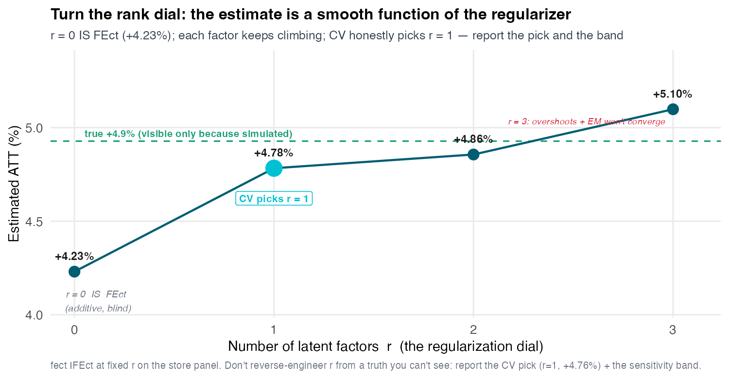
The cleanest picture of “the method is the regularizer” is the rank dial (Figure 17.9): refit IFEct at fixed $r=0,1,2,3$ and plot the ATT against $r$. At $r=0$ the estimate is exactly the FEct number, +4.23% — the dial at zero reprints the additive imputation, so the whole nesting is visible in one line. Turn it: $r=1$ gives +4.78%, $r=2$ +4.86%, $r=3$ +5.10% — a smooth, climbing function of the regularizer, and by $r=3$ it overshoots the truth and the EM algorithm stops converging (over-ranked, poorly conditioned). Two numbers live near each other here and they are not the same: the dial’s $r=1$ is +4.78%, a fixed-$r$ refit, while the headline IFEct estimate is +4.76%, the CV-selected fit — different EM runs at the same rank. Quote +4.78% on the dial and +4.76% as the answer.

You stop the dial without the truth line by cross-validation — and it is worth being exact about what fect actually does, because the usual one-line description of CV is wrong in two ways. It does not scatter blanks across the panel. Under its default cv.method = "rolling" it samples 10% of the stores, hides a contiguous three-week block of their observed pre-launch weeks, and deletes everything after that block from the training window — so the model must forecast forward onto cells it was denied. That geometry is deliberate: it mimics the shape of the real imputation job (fit on the pre-period, extrapolate into the post-period) rather than filling scattered interior holes. And the keep-rule is not the argmin: fect’s default cv.rule = "1se" keeps the simplest model whose held-out error lies within one standard error of the best. On BeanBuzz that is $r=1$ — a second factor does not improve held-out prediction enough to earn its place, because $F_2$ is weak. (You will see the 1-SE rule bite in Section 17.3.4.7, where it rejects matrix completion’s lowest-scoring $\lambda$.) The discipline point, which A5 rewards: you report what CV gave you (+4.76% at $r=1$), not the oracle-informed $r=2$ (≈ +4.9%), because a practitioner has no truth line to reverse-engineer the factor count from. The small residual gap between the $r=1$ estimate and the truth is not a bug to fix by peeking — it is the honest cost of not knowing how many factors the world has.

Be clear about what this dial is, because it is easy to mistake it for something it is not. Turning the rank knob is model selection — it answers “which rung fits best?” It is not a stress test of an assumption, and it is not a sensitivity band. What the rung you picked still cannot see, and what that blindness costs, is a different question entirely: that is Section 17.3.5.

Figure 17.9: Estimated ATT plotted against fixed rank r on the store panel: r=0 is FEct at +4.23, r=1 the fixed-rank refit at +4.78 (the CV-selected fit is +4.76), r=2 at +4.86, r=3 at +5.10 overshooting the true +4.93 line and failing to converge. The true line is dashed and labelled “visible only because simulated.”

17.3.4.5 +4.76% is the average of a ramp — not a level

Now draw the answer instead of quoting it. plot(out.ife) — one bare call on the CV-selected fit — and the headline stops being a number and becomes a path (Figure 17.10):

out.ife <- fect(log_rev ~ app_live, data = df, index = c("sid", "week"),
                method = "ife", CV = TRUE, r = c(0, 5), force = "two-way",
                se = TRUE, nboots = 200)
plot(out.ife, main = "Estimated ATT (IFEct)")

Table 17.2: The effect ramps. Adoption is a diffusion, not a switch: in the launch week the app is barely installed, and a year in it is worth +6.58%.

event week	1	4	8	12	26	52
ATT	+0.75%	+2.49%	+3.86%	+4.25%	+5.65%	+6.58%

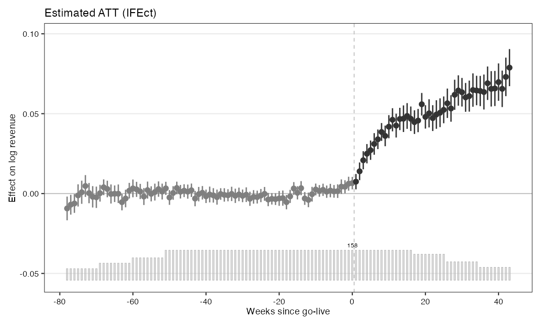
Figure 17.10: `plot(out.ife, main = "Estimated ATT (IFEct)")` — the CV-selected IFEct event study, with 200-draw bootstrap bands. Flat before go-live; a saturating ramp after. The headline **+4.76%** is the *mean of the black points to the right of the dashed line*.

The headline is a mean over a window YOU chose — and the window is a choice

+4.76% is not “the effect of the app.” It is the average of that ramp over the post-window this panel happens to contain. Change the window and you change the number, with no error anywhere:

over weeks 1–12 the same path averages +3.04%
at week 52 alone it is +6.58%
the reported headline, averaging every post cell, is +4.76%

All three are correct. They answer different questions, and fect will print whichever one you ask for without a warning. A board asking “what will this be worth next year?” wants +6.58%; a board asking “what did the first quarter buy?” wants +3.04%. Quoting the headline to either is wrong.

This is the same blade as Section 17.3.6’s calendar plot, arriving early: the aggregation is the question. It is also the trap S10 sprang and the reason Section 17.3.5 insists you name what a robust interval bounds — the sweeps there bound the 12-week mean (+3.13% on the placebo fit), not the +4.76% headline.

And read the left half of Figure 17.10 with equal care, because it is doing quiet work: the pre-launch points sit flat on zero. That flatness is not reassurance — it is a claim, and it is precisely the claim Section 17.3.5 spends four tests auditing. (It does not survive intact: the placebo fires at +0.78 pp.) A flat pre-trend on a picture is a hypothesis, not a certificate.

17.3.4.6 Same panel. Same picture. A different number.

Now run the other family on the same panel and plot it the same way. plot(out.mc) (Figure 17.11) — and put the two event studies side by side.

They are visually indistinguishable. Flat before, ramping after, same curvature, same bands. That is not an impression; it is measured: the two ATT paths correlate 0.988 over the post-launch weeks and 0.998 over the full window, and the largest gap at any single post week is 0.97 pp.

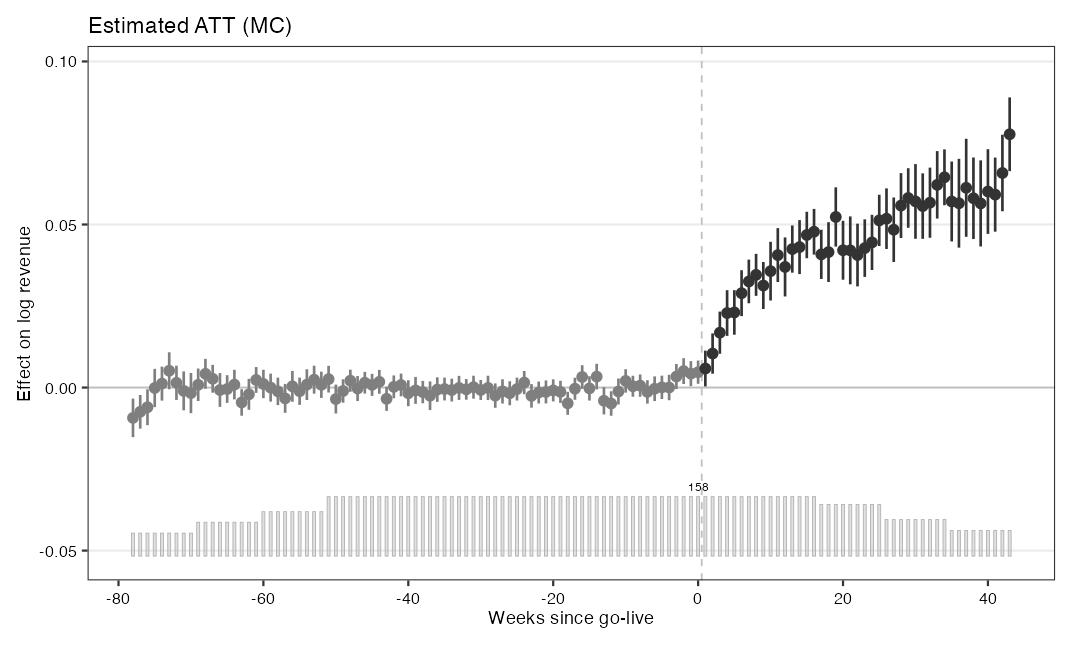
Figure 17.11: `plot(out.mc, main = "Estimated ATT (MC)")` — matrix completion on the identical panel, identical plot call. Compare it with Figure 17.10: the shape is the same. Only the number is not.

Table 17.3: Two models, one panel, two answers — and each interval contains the other’s point estimate.

estimator	ATT	S.E.	95% CI
IFEct (hard-impute, $r=1$)	+4.76%	0.27 pp	[+4.23, +5.28]
MC (soft-impute, nuclear norm)	+4.31%	0.30 pp	[+3.73, +4.89]

Nothing you can SEE separates them

Look at what those intervals do. MC’s CI comfortably contains IFEct’s estimate; IFEct’s comfortably contains MC’s. The entire quarrel — 0.45 pp — is smaller than a single CI half-width (IFEct’s alone is 0.53 pp). The disagreement between the two models is smaller than the noise inside either one of them.

So nothing visible chooses: not the fit to the observed cells (identical by construction — that is what fitting does), not the shape (correlation 0.988), not the intervals (overlapping across nearly their whole length). Hand a board these two event studies with the titles removed and no one can tell you which is which.

The 0.45 pp lives entirely on the grey cells — the imputed $Y(0)$ for treated store-weeks — which is exactly where no picture can go, because there is nothing there to plot.

And refuse the two cheap escapes. (a) “The CIs overlap, so it doesn’t matter.” Wrong twice: overlapping intervals are not a test of equality, and the question is not significance — it is which imputation is right, on which the CI is silent. (b) “Just take the more flexible model.” Hold that thought for two subsections: MC is the more flexible tool and it under-recovers (Figure 17.12).

⇒ If neither the picture nor the interval can choose, what can? That is the question Section 17.3.4.7 answers — and the honest answer is that cross-validation can rank, and still cannot acquit.

17.3.4.7 The same folds also rank the families — and they do it with no truth line

The dial answers “which rung of the IFEct ladder?”. But the deeper question a practitioner faces is “which family — hard-impute (IFEct, tune $r$) or soft-impute (MC, tune $\lambda$)?” — and it is the one you cannot answer by peeking, because you have no answer key. Cross-validation answers it too, and fect will do it for you in one argument:

fect(log_rev ~ app_live, data = df, index = c("sid", "week"),
     method = "both",        # <- race BOTH families on ONE set of folds
     CV = TRUE, r = c(0, 5), nlambda = 10, k = 5, force = "two-way")

method = "both" is not a fourth estimator. It builds the held-out folds once — before it branches to either family — then runs the whole $r$-ladder and the whole $\lambda$-ladder over those same hidden cells. On BeanBuzz (set.seed(20260713), $k=5$) the two ladders come back like this, both scored on the same 345 held-out cells:

$r$ (IFEct)	held-out MSPE	$\lambda/\sigma_{\max}$ (MC)	held-out MSPE
0	0.00171 (= FEct)	1.00	0.00171 (= FEct)
1	0.00105 ← kept	0.42	0.00149 ← kept
2	0.00116	0.18	0.00137 ← lowest
3	0.00118	0.075	0.00149
4 · 5	0.00154 · 0.00199	0.032 · 0.013	0.00160 · 0.00166

fect then prints its own verdict — Recommended method through cross-validation: ife — and hands back $r=1$, +4.76%: the headline, reached with no oracle anywhere in the calculation.

Three things in that table are worth more than the verdict.

(1) The first row is a receipt, not a coincidence. Both ladders nest FEct: IFEct at $r=0$ is the additive imputation, and MC at $\lambda = \sigma_{\max}$ shrinks every singular value to zero and is the additive imputation too (that is the “nested, to the boundary” point from the previous section, cashed out). Same model, two entrances — so if and only if the two ladders were scored on the same hidden cells, those two rows must report the same number. They do, to the last bit: 0.001713945337004485 on both, identical() returns TRUE. That equality is the proof the comparison is legitimate.

Never compare two separately-fitted MSPEs

fect’s seed= argument seeds the bootstrap, not the cross-validation. If you call fect twice — once with method = "ife", once with method = "mc" — the two calls draw their folds from the ambient RNG stream one after the other and therefore hold out different cells. On this panel the two fold sets share 3 cells out of ~345: they are essentially disjoint. And the cost is not small. The same model — FEct — scores 0.00171 on one fold set and 0.00187 on the other: a 9% gap produced by nothing but which cells got hidden, the same size as the real gap between the two families. Two separately-fitted MSPEs side by side are a race on two different racetracks, and the noise is as large as the signal. Use method = "both", or reset set.seed() immediately before each call.

(2) MC keeps $\lambda/\sigma_{\max} = 0.42$, not its lowest-scoring $0.18$. “Keep the lowest held-out error” is not what the package does. fect’s default is cv.rule = "1se": keep the simplest model whose error is within one standard error of the best. Here the difference between 0.00137 and 0.00149 is 0.00012 against a standard error of 0.00019 — not a difference at all — so fect rejects the winner, prints [cv.rule = 1se] lambda.cv adjusted (1-SE band), and takes the more-shrunken model. When the data cannot tell two models apart, the regularized one is the defensible one.

(3) The ranking is strong, but it is not a proof. IFEct’s best (0.00105) beats MC’s best (0.00137) by ~24%, a gap 3.1× IFEct’s own fold standard error. Re-run the race on 30 different fold draws and CV picks IFEct on 29 of them (97%; 95% CI 83–100%). On one draw it picks MC and hands back +4.31% instead. So say “CV prefers IFEct here, on almost every fold draw” — never “CV settles it.”

And now the refusal, which is the whole point. Every one of those 345 held-out cells is an observed, pre-launch week — 23 stores per fold, a contiguous three-week block each, with everything after the block deleted from training so the model must forecast forward. That design is the best defence of the exercise: it mimics the shape of the real job rather than filling scattered interior holes. But it cannot close the gap that matters. The estimand needs $Y(0)$ on treated, post-launch cells — for stores that selected into treatment, at event times with no observed counterpart. Cross-validation never scores one of those, and it never can: they are precisely the cells that do not exist. A model can win this race and still impute the counterfactual worse.

Held-out fit can RANK the candidates. The placebo can CONVICT one. Nothing can ACQUIT.

The very next result shows what that costs — and it is not an abstraction.

17.3.4.8 Seeing the factor lifts the estimate — but more flexible $\neq$ more right

Once the model sees that wave and lets stores load on it differently, the imputed $Y(0)$ bends correctly, the downward bias from averaging the factor away disappears, and the estimate climbs (Figure 17.12). The additive family is blind to it and undershoots — static two-way FE +3.7%, Callaway-Sant’Anna +3.3%, the FEct imputation +4.23% (note the additive estimators are not even monotone among themselves). The moment interactive fixed effects sees the factor, IFEct climbs to +4.76% — recovering most of the gap to the true +4.93%. The factor family does what the additive family could not: it closes the structural gap. IFEct is the hero — the estimator that recovered the factor and the truth together. (The naive pre/post +16.3% is off the ladder entirely: it is selection, not an estimator to rank.)

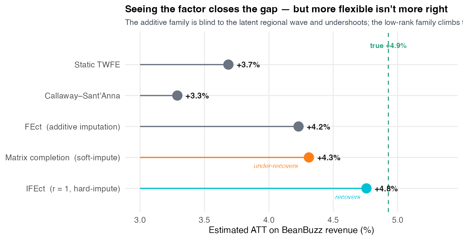
Figure 17.12: A lollipop of point estimates in two clusters. The additive family — static two-way FE +3.7, Callaway-Sant’Anna +3.3, FEct +4.23 — sits below the true +4.93% line; the low-rank family climbs, with matrix completion +4.31 flagged as under-recovering and IFEct +4.76 as recovering. fect only, no gsynth.

Now the discipline lesson, which is non-negotiable. Matrix completion, the most flexible tool on the ladder, lands at +4.31% — barely above the additive number, under-recovering the truth. Why? Its nuclear-norm penalty shrinks the singular values toward zero, and in doing so it shrank the very factor we needed to recover — the penalty that buys flexibility also dampened the signal. The lesson, in five words: more flexible is not more right. Flexibility is not free; it must be tuned, not assumed. A bigger hypothesis space can under-fit the truth if its regularizer pulls the wrong way. Do not leave thinking matrix completion recovered the truth — it did not. This is the honest counterweight to the seductive “just use the most powerful method” instinct, and exactly the judgment A5 rewards.

17.3.5 Sensitivity analysis

17.3.5.1 Low rank does not delete parallel trends — it demotes it

Before the first diagnostic, dissolve the objection you should already be feeling. The ledger says S12 replaced parallel trends with low rank; the deck’s climax was that +4.23% is blind, not biased. So why spend an act stress-testing parallel trends — the assumption we just escaped?

Because the dial’s bottom rung is the imputation DiD. We proved it to the digit in Section 17.3.3: at $r=0$, FEct = BJS = the hand-rolled recipe = +4.23%. At $r=0$ you are assuming parallel trends exactly, not approximately — so whatever stress test that estimator needs, the bottom rung needs. (Be precise about what the identity says: FEct equals the BJS/hand-rolled imputation on this panel. It does not equal Callaway–Sant’Anna, which lands at +3.3%. “$r=0$ is DiD” means “$r=0$ is the imputation DiD,” and that is all it means.)

And above the bottom rung the assumption is not deleted — it is demoted. IFEct still needs its imputed $Y(0)$ to be right on the grey cells, and it will be right only if the factor structure it fitted actually captured the drift. Whatever the model failed to absorb — an omitted second factor, anticipation, a genuine differential trend — reappears as a violation path $\delta_t$ in the residual. Parallel trends went from “the raw panel moves in parallel” to “the panel moves in parallel once $\Lambda F$ comes out”; for MC, once the shrunken singular values come out. That is good news, not bad: a demoted assumption is a measurable one, and the residual is exactly what a placebo can put a ruler on.

From here on: no answer key

Everything up to this point leaned on a truth line, because we built BeanBuzz and could. From this section to the end of the session, that stops. The rank is fixed at the CV pick, $r=1$ — no dial, no rung comparison — and every claim below is derivable from what fect prints on your own screen. You will never have an answer key again; the point of the next two sections is what you do without one. One question now runs the act: how much unabsorbed drift can this fit’s answer survive?

17.3.5.2 Four tests, four nulls, no verdict

The act runs four tests on the same fit — IFEct at the CV-selected $r = 1$. They are not four attempts at one question. They ask four different questions, they have four different nulls, and two of them disagree with each other. That disagreement is the finding.

Table 17.4: Four tests, four nulls. Tests 3 and 4 price the same violation in two currencies — and return opposite verdicts.

#	test	what it asks	on this fit
1	Placebo	Blank three pre-weeks the model would have learned from. How badly does it re-impute them?	fires ($p=0.002$) and is small (TOST $p=0.005$) — and hands back a ruler, 0.240 pp
2	Leave-one-out	The pre-trend looked flat — but the model was fitted on it. Re-impute every pre-period out of sample.	TOST 0.082 → 0.350. Nothing certifies.
3	Relative magnitudes	Bound the post-launch violation by the pre-launch drift. How much can the answer take?	survives to $\bar M^{} = 0.46$ — 0.11 pp/week*
4	Smoothness	Bound the curvature instead. Same question, different belief about the violation’s shape.	*dies at $M^{} = 0$**

Nothing here will produce a verdict. Tests 1 and 2 measure the violation; Tests 3 and 4 price it. The question “did the pre-trends pass?” has no answer, and by the end of the act you will be able to say precisely why.

17.3.5.3 Test 1 — the placebo hands back a path, not a pass

Every pre-period effect you have seen so far was a cell the model fitted. Of course they looked flat — that is what fitting does. The placebo blanks cells the model is denied:

out.p <- fect(log_rev ~ app_live, ..., method = "ife", r = 1,
              placeboTest    = TRUE,
              placebo.period = c(-2, 0))

plot(out.p, stats = c("placebo.p", "equiv.p"))

That blanks the three pre-treatment cells at $e = -2, -1, 0$ and re-imputes them out of sample, from a model that never saw them. It is a pre-trend test applied to the imputation itself, and it is the only test in this session the estimator could actually fail (Figure 17.13).

fect prints two p-values on that figure, and they answer two different nulls:

Table 17.5: Both nulls are rejected. Both rejections are correct.

test	its null hypothesis	on this fit	a rejection means
t-test	$\text{ATT} = 0$ on the blanked window $\{-2,-1,0\}$	0.002	rejects → the violation is real
TOST (two one-sided tests)	$\lvert\text{ATT}\rvert \ge \theta$, with $\theta = 1.44$ pp	0.005	rejects → the violation is small

It failed — placebo ATT +0.78 pp, $p = 0.002$. And it passed — placebo equivalence $p = 0.005$: the same three cells are significantly small.

Both p-values are printed by fect. Both are correct. Significance is not size.

With 158 treated stores, a residual worth one-sixth of the effect clears $p < 0.05$ with room to spare — while also being provably smaller than any threshold you would call meaningful. Anyone still holding a pass/fail gate has just watched it open and close at the same time. So throw the gate away and keep what the placebo actually handed back.

Where does $\theta = 1.44$ pp come from? Nobody in this room chose it.

The TOST needs a bar: how small is small enough? fect sets it as

\[\theta \;=\; 0.36 \times \sqrt{\texttt{sigma2.fect}}\]

and it is worth walking that in plain language, because three separate choices are buried in it.

How noisy is a store-week, normally? Fit a plain two-way fixed-effects model — store effects plus week effects — and take the standard deviation of what is left over. On the placebo fit that is 3.99 pp of log revenue. That is the everyday wobble of a store-week once the store’s level and the week’s common shock are removed.
Multiply by 0.36. This is fect’s hard-coded convention for small: roughly a third of a typical wobble.
That is the bar. $0.36 \times 3.99 = \mathbf{1.44}$ pp.

Now the three things that should bother you.

The bar was cut from the wrong model’s noise. $\texttt{sigma2.fect}$ is the residual MSE of the baseline two-way-FE model — 3.99 pp. But the model under test is IFEct, whose own residual SD is only 3.05 pp: the factor absorbs real variation, so IFEct is quieter than the baseline. It is being graded against a noisier model’s yardstick, which makes the bar roughly 30% more generous than its own noise would justify.
Nobody declared the 0.36. It is a package default, not a standard you set and defended.
“Negligible” here means “up to half the effect.” 1.44 pp is 46% of the +3.13% this test would be certifying.

And note that $\theta$ is a property of a fit, not of a session: the plain fit’s bar is 1.43 pp (0.36 × 3.97), because blanking three weeks nudges the baseline MSE. That is the number you will see in Test 2. Same formula, different fit, different bar — quote the one that belongs to the object you called.

What the placebo actually handed back is a path — the imputation’s own error in each blanked week:

\[\delta_{-2} = +0.62 \text{ pp} \;\longrightarrow\; \delta_{-1} = +0.86 \text{ pp} \;\longrightarrow\; \delta_{0} = +0.88 \text{ pp}\]

and its two consecutive first differences — the change from one week to the next — of 0.240 pp and 0.018 pp. The larger of those is the object the whole rest of the act is denominated in:

The ruler $R$ = 0.240 pp — the largest step inside the blanked window. A step, not a level.

Two details separate a careful analyst from a careless one. The cell at $e=-3$ is one the model trained on — an in-sample fit residual, not a held-out imputation error — so fect_sens() never sees it and it is not part of the benchmark. And what is bounded is the step: that distinction is the entire content of Tests 3 and 4, so plant it now.

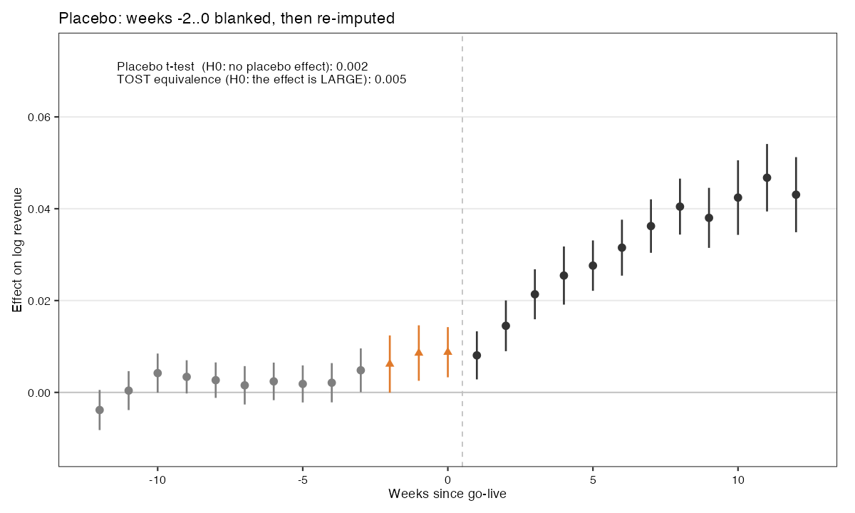
Figure 17.13: `plot(out.p, stats = c("placebo.p", "equiv.p"))`. The three orange placebo points at event weeks −2, −1, 0 are cells blanked and re-imputed out of sample. `fect` prints both verdicts on the figure: the placebo test (p = 0.002 — it fires) and the placebo *equivalence* test (p = 0.005 — it is significantly small). The path rises +0.62 → +0.86 → +0.88 pp across the blanked window.

The ruler has an error bar, and it is bigger than the ruler

The two steps carry standard errors of 0.283 and 0.240 pp — larger than the quantities they estimate — and the ruler’s own bootstrap 95% CI runs [0.07, 0.75] pp, an eleven-fold range. Use it — you have no other — but never quote it to three digits, and never let a manager hear it as a measurement.

And name $\delta_0$ honestly. Calling it “the model’s own imputation error” is true only under no anticipation: a pre-launch marketing push would look identical on this figure, and nothing on your screen separates the two. Say “whatever $\delta_0$ is.” Never say “the bias.”

(Why weeks $-2 \ldots 0$? It is fect’s documented default, and it is the window immediately adjacent to treatment — the hardest to impute, and therefore the most honest ruler. Widen it and the ruler changes. That is a researcher degree of freedom like any other: declare it.)

17.3.5.4 Test 2 — leave-one-out: the model grades its own homework

Start where everyone starts: the pre-trend plot. plot(f, type = "equiv") draws the pre-period effects with two bands — a grey Min. Range (the widest the pre-period estimates actually get) and a red Equiv. Range (the bar from Test 1, here 1.43 pp, because this is the plain fit) — and prints its verdicts in the corner (Figure 17.14).

fect computes three tests on every fit and shows only two unless you ask. Ask:

plot(f, type = "equiv", stats = c("F.p", "F.equiv.p", "equiv.p"))

Table 17.6: Three tests, three different nulls, one fit — and fect hides the only one that certifies.

test	its null hypothesis	on this fit	what a rejection means
F test	there is no pre-trend	0.126	cannot reject → absence of evidence
F-equivalence	the pre-trend is large	0.019	rejects → it certifies
TOST	some pre-period is large	0.082	cannot reject → it does not certify

Read them in order. The F test at $p = 0.126$ says only that we cannot reject “no pre-trend” — and this course has policed that fallacy since S03. Nobody may say “the pre-trends passed.” The F-equivalence test at $p = 0.019$ is the one that can license the word small: its null is that the violation is large, and we reject it. It is computed on every fit you have ever run and never shown. The TOST at $p = 0.082$ does not certify — and it is not contradicting the others: TOST is an intersection-union test, so every tested pre-period must individually clear the bar, and it therefore reports the worst one. Here the worst is event week $-78$, a thin cell holding only 61 of the 158 stores. Do not dismiss that as low power: the point estimate supplies about 61% of the 1.52 pp Min. Range and the standard error only 39%. It is a real bump in a thin cell.

Nobody chose the band, and nobody chose the window

proportion is fect’s rule for which pre-periods are tested at all — the default keeps periods observed for at least 30% of treated units. Raise it to 0.5. One argument. Same fit, same call, same data (Figure 17.15). Week $-78$ leaves the window, the grey Min. Range walks from ±1.52 pp to ±1.00 pp and crosses the red line, and TOST goes 0.082 → 0.000. The same panel now certifies its own pre-trend.

This is not a trick for passing pre-trend tests, and it is not licence to run both and report the one that survives. Neither 0.3 nor 0.5 is right. It demonstrates that the verdict is a choice nobody made: the window came from a default you never read, and it decides whether the panel certifies at all; the band is the $\theta$ you met in Test 1, cut from a different model’s noise.

So the question “did the pre-trend pass?” has no answer. Replace it with the one that does: how big a violation would it take to kill my answer? That is a price, and Tests 3 and 4 pay it.

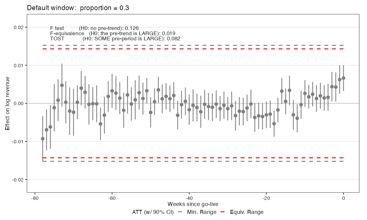
Figure 17.14: `plot(f, type = "equiv", stats = c("F.p","F.equiv.p","equiv.p"))` at `fect`’s default window. The grey Min. Range band (±1.52 pp) sits **outside** the red Equiv. Range (±1.43 pp), and the three printed p-values are F 0.126, F-equivalence 0.019, TOST 0.082.

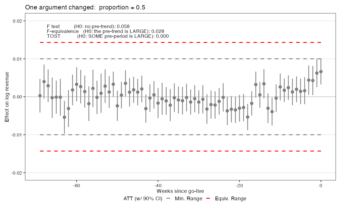
Figure 17.15: The identical call with `proportion = 0.5`. Event week −78 — a thin cell holding 61 of 158 stores — leaves the tested window; the grey Min. Range falls to ±1.00 pp and now sits **inside** the red Equiv. Range, and TOST goes 0.082 → 0.000. The same panel certifies its own pre-trend.

But every number above is in-sample. The model was fitted on those pre-period cells. A flat pre-trend computed in-sample is not evidence of parallel trends; it is partly a receipt for having run a regression. Remove the circularity — for every pre-period $t$, refit without $t$, then impute $t$:

out.loo <- fect(log_rev ~ app_live, ..., method = "ife", r = 1,
                loo = TRUE)

plot(out.loo, type = "equiv", loo = TRUE)

Eighty-eight refits (one per pre-period), of which 79 clear the proportion filter and are tested. Genuinely out-of-sample pre-period estimates (Figure 17.16). Now read the table across, and note which numbers move and which do not:

Table 17.7: Two tests shrug. One collapses.

$p$-value	its null	in-sample	LOO
F	no pre-trend	0.126	0.147
F-equivalence	the pre-trend is large	0.019	0.015
TOST	some pre-period is large	0.082	0.350

The F tests barely move, and F-equivalence still certifies. TOST quadruples. That is not a puzzle — it is the two tests’ arithmetic. The F tests are averages over the pre-periods, and averages are forgiving: a few bad weeks are diluted by eighty good ones. TOST is intersection-union — every pre-period must individually clear the bar — so it reports the worst of 79. In-sample the worst week was borderline. Out of sample it is not close.

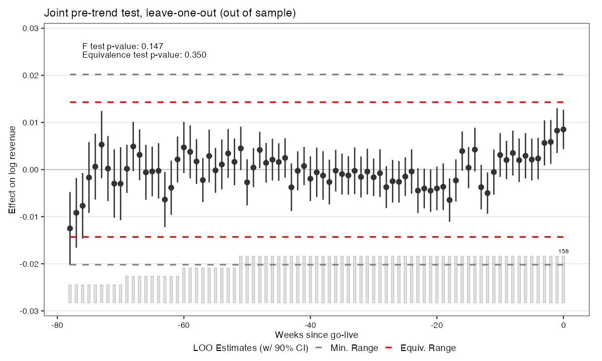
Figure 17.16: `plot(out.loo, type = "equiv", loo = TRUE)`. Each pre-launch week is re-imputed from a model that never saw it. The grey Min. Range walks out to ±2.02 pp, well outside the red ±1.43 pp Equiv. Range. Printed: F = 0.147, equivalence = 0.350.

Say it precisely: LOO did not flip a pass into a fail

The tempting sentence is “out of sample, the pre-trend crossed the line.” It is wrong, and a student with the previous figure in hand will catch you. The grey Min. Range was already outside the red bar in-sample — 1.52 pp against a 1.43 pp bar — which is exactly why the in-sample TOST was 0.082 and never certified at 5% either. Out of sample the grey walks to 2.02 pp.

LOO widens a failure that was already there, from marginal to decisive. And the conclusion is not “the pre-trend failed” — that is the same fallacy in the other direction. The honest report is: nothing here certifies the pre-trend, the model’s out-of-sample pre-period behaviour is materially worse than its in-sample behaviour, and the in-sample number was hiding exactly that.

fect defect: the plot prints one pair of numbers and returns another

Ask the LOO plot for its statistics with return.test = TRUE and you get the cached in-sample test.out — F 0.126, TOST 0.082 — not the out-of-sample numbers the figure just printed (0.147, 0.350). Those live in a different slot: out.loo$loo.test.out.

This is the second time this package has handed back a stale object (the same trap fires on plot(type = "equiv", return.test = TRUE) for the plain fit, where fect() stores f.threshold = 0.5 — the figure’s 0.019 — while the internal fect:::diagtest() helper defaults to 0.6, the object’s 0.005). Rule: if you quote a number a package printed on a figure, get it from where the figure got it.

(And never pass xlim= to type="equiv": it recomputes the grey Min. Range over the plotted window but not the printed p-value, so you get a passing picture beside a failing statistic. Use proportion=, which recomputes both.)

17.3.5.5 Test 3 — relative magnitudes: $\bar M = 0$ is not innocence, it is frozen

Two tests have now measured the violation. Neither said what it costs. The relative-magnitudes restriction (Rambachan and Roth 2023), implemented for counterfactual estimators as fect_sens() (Chiu et al. 2026), replaces the binary pre-test with a continuous sensitivity analysis. Let $\delta_t$ be the violation path — the observed coefficient is effect $+\ \delta_t$, and identification fails precisely because you cannot separate them. Then

\[\Delta^{RM}(\bar M) = \Big\{\delta:\ \big|\delta_{t+1}-\delta_t\big| \le \bar M \cdot \underbrace{\max\big(|\delta_{-1}-\delta_{-2}|,\ |\delta_0-\delta_{-1}|\big)}_{R \;=\; \text{the ruler} \;=\; 0.240\text{ pp}},\ \forall t \ge 0\Big\}\]

In words: after launch, the violation may not move faster, week to week, than $\bar M$ times the fastest it moved where we could watch it. That is why Test 1 had to come first — the denominator is its ruler.

s <- fect_sens(out.p, post.periods = 1:12,
        Mbarvec       = seq(0, 1, 0.05),
        periodMbarvec = c(0, 0.5))

plot(s, type = "sens",    restrict = "rm")   # the 12-week ATT
plot(s, type = "sens_es", restrict = "rm")   # period by period

Each $\bar M$ yields a robust C-LF confidence interval; the breakdown $\bar M^{*}$ is the smallest $\bar M$ whose interval first covers zero (Figure 17.17).

Name the object — a robust CI is meaningless without it

The sweep bounds the mean effect over post-weeks 1–12 = +3.13% — the 12-week ATT of the placebo fit — with an original (uncorrected) band of [+2.73%, +3.52%]. It does not bound the +4.78% headline. The effect is a saturating ramp, so a twelve-week average sits well below the matured plateau. S10 hit exactly this trap. Never quote a robust interval without naming what it bounds.

Now look at the first two bars and ask the question the figure poses and does not answer:

If $\bar M = 0$ means “assume no violation,” why is the $\bar M = 0$ band centred +0.88 points below the original — a shift bigger than the original band is wide?

Table 17.8: The $\bar M = 0$ set does not sit inside the original — it sits below it.

	95% set, 12-week ATT	centre
Original (uncorrected)	[+2.73%, +3.52%]	+3.13%
$\bar M = 0$	[+1.61%, +2.89%]	+2.25%

A null assumption cannot move an estimate. So $\bar M = 0$ is not the null. $\Delta^{RM}(0)$ is the set of violation paths whose consecutive differences are bounded by zero — the violation may not change. It does not say the violation is zero; it says it is constant. And it is constant at the last thing we measured: $\delta_0 = +0.88$ pp, the final blanked cell. Do the arithmetic:

\[3.13 - 0.88 = 2.25\]

fect calls the result a de-biased interval, and that is telling you the exact truth: it froze a violation and subtracted it from every post-week. Not unbiased — de-biased. And it charges for it: the band is 61% wider (0.79 → 1.28 pp), because $\delta_0$ is estimated and the extra width is the standard error of the thing you just subtracted.

Same notation. Different vector. Opposite meaning. (Pay the S10 debt.)

Your instinct that $\bar M = 0$ means exact parallel trends is not stupid — this course installed it, and it was correct where you learned it. In S10, HonestDiD ran on an event study with an omitted base period, so $\delta_{-1} \equiv 0$ by construction; there $\bar M = 0$ genuinely was exact parallel trends, and S10’s $\bar M = 0$ CI sat centred on its original, exactly as an omitted base period predicts.

An imputation estimator normalises nothing. Every pre-period coefficient is freely estimated, so $\delta_0$ is a real, non-zero number — and zero freezes it. Same notation. Different vector. Opposite meaning.

$\bar M^{*} = 0.46$ — of what? On the 0.05 grid the lower bound first covers zero at $\bar M^{*} = 0.50$. Refine the grid to 0.01 (Mbarvec = seq(0.40, 0.55, 0.01)) and the crossing is at 0.46: the lower bound is $+3.6\times10^{-4}$ at 0.45 and $-4.0\times10^{-5}$ at 0.46. Report 0.46 — and say that the coarse grid rounded your robustness up by 9%. On a topic whose thesis is name your hidden choices, the grid resolution is one of them, and you got it for free.

Now the sentence that matters, and it must be said as a pair:

$\bar M^{*} = 0.46$ — which on this fit is about 0.11 percentage points of drift per week ($0.46 \times 0.240$ pp).

Never the first half alone. Look at the x-axis of Figure 17.17: $\bar M$ is unitless. It is a multiple of a ruler this model cut out of its own residual.

A model that fits its pre-window better earns a bigger $\bar M^{*}$ — for free

A better pre-fit cuts a shorter ruler, and a shorter ruler makes every $\bar M$ cheaper — so the breakdown value rises mechanically, rewarding the model for being better at hiding its own error. $\bar M^{*}$ is denominated in what your model still cannot see.

Never compare a bare $\bar M^{*}$ across models, panels, or sessions. S10’s HonestDiD sweep on this same firm broke at $\bar M^{*} = 0.25$. S12 is not “twice as robust as S10.” Different fit, different object, different ruler — the two numbers are not even in the same units. The honest report is always the pair.

And $\Delta^{RM}$ bounds the step, so the level accumulates — which is what the period-by-period sweep shows (Figure 17.18). At $\bar M = 0$, 2 of the 12 post-weeks already contain zero; at $\bar M = 0.5$, 9 of 12 do — even though the twelve-week average has not quite broken. The sets widen with the horizon, because a step allowance compounds the further out you go: week 12 is far more fragile than week 3, and at the breakdown price the violation can reach $\delta_0 + 12 \times 0.11 \approx$ 2.2 pp by week 12, against a +3.13% effect. Aggregation hides fragility, and a per-week number quoted with no horizon is worse than useless.

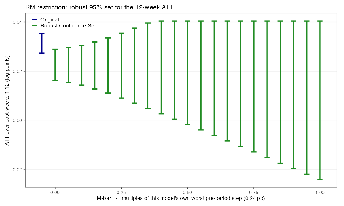
Figure 17.17: `plot(s, type = "sens", restrict = "rm")` — the RM sweep at $r=1$. The robust 95% C-LF set for the 12-week ATT against $\bar M$. The lower bounds fall steadily and first cover zero at $\bar M = 0.46$; the upper edge goes dead flat at +4.04% from $\bar M = 0.40$ rightward — that ceiling is HonestDiD’s $20\times\text{SE}$ search grid, **not a bound**.

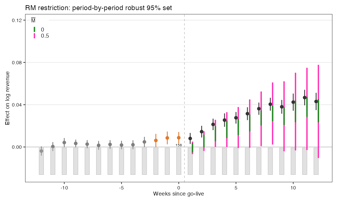
Figure 17.18: `plot(s, type = "sens_es", restrict = "rm")` — the same restriction, period by period. Green is $\bar M = 0$, pink is $\bar M = 0.5$. The sets widen with the horizon: 2 of 12 weeks contain zero at $\bar M = 0$, and 9 of 12 at $\bar M = 0.5$.

The lid: a package defect that changes a number

Look at the top edge of Figure 17.17 from $\bar M = 0.40$ rightward. It is dead flat. That is not a bound — it is HonestDiD’s default search-grid ceiling, $20 \times \text{SE} = +4.0394\%$, and 13 of the 21 upper bounds are pinned to it to eight decimal places (on the refined grid, all 21 are). When the true bound lies outside its grid, HonestDiD warns — and fect_sens() swallows that warning (“CI is open at one of the endpoints”) inside suppressWarnings().

A robust set must widen strictly in $\bar M$. A constant upper bound across thirteen consecutive grid points is not econometrics, it is truncation. The upper edge is censored, not bounded.

Rule: treat every fect_sens upper bound as censored until you have checked it against $20\times\text{SE}$. Here the lower bounds are clean — 0 of 21 pinned — which is the only reason $\bar M^{*}$ survives at all. Report the lower bounds; do not print the upper ones.

(A cosmetic cousin, so you are not caught by it: plot(type = "sens") is hardcoded with the title “Smoothness Restriction Sensitivity Analysis” for both values of restrict. main= is mandatory. Believe the axis, not the title.)

17.3.5.6 Test 4 — smoothness: it dies at $M^{*} = 0$

The smoothness restriction bounds the second difference — the curvature — instead of the step:

\[\Delta^{SD}(M) = \Big\{\delta:\ \big|(\delta_{t+1}-\delta_t)-(\delta_t-\delta_{t-1})\big| \le M,\ \forall t\Big\}\]

s <- fect_sens(out.p, post.periods = 1:12,
        Mvec       = seq(0, 0.010, 0.002),
        periodMvec = c(0, 0.004))

plot(s, type = "sens_es", restrict = "sm")

$M = 0$ forces $\delta$ to be a straight line — which is emphatically not $\delta = 0$. A violation growing by the same amount every week for twelve weeks is perfectly linear and perfectly legal inside $\Delta^{SD}(0)$: $M = 0$ forbids acceleration, not bias. Note also the practical burden — $M$ is in log points, so you must supply it in the outcome’s own units, whereas $\bar M$ is unit-free. That is a large part of why A5 asks for relative magnitudes.

RM and SD both have a setting called “zero,” and the two zeros assume opposite things. RM-zero says the violation never changes. SD-zero says it changes at a perfectly constant rate. Same name; opposite content. Fed the identical fit, they return opposite verdicts:

Table 17.9: At its strictest setting the smoothness set already covers zero. $M^{*} = 0$.

$M$	robust 95% set, 12-week ATT
0.000	[−1.10%, +4.04%]	← contains zero
0.004	[−12.77%, +16.17%]
0.010	[−30.93%, +34.37%]

$M^{*} = 0$: under smoothness, this estimate has no robustness at all — not the average, and not a single week. The period-by-period sweep (Figure 17.20) puts 12 of 12 post-weeks over zero at $M = 0$.

RM survives to 0.46. Smoothness dies at 0. Same panel, same fit, same estimand.

$\Delta^{SD}(0)$ does not say “there is no violation.” It says the violation is a straight line — and a line fitted to a noisy pre-window and run out twelve weeks eats the whole effect.

That is the difference between the two restrictions, and it is the whole act:

$\Delta^{RM}$ bounds a step. A step allowance accumulates linearly.
$\Delta^{SD}$ bounds a bend. A bend accumulates quadratically — by week 12 at $M = 0.004$ the set is [−33.0%, +39.4%], for an effect of +4%.

You cannot test which is right. The violation lives on the grey cells, and the grey cells are the ones you never see. That is the definition of the problem, and no sweep, no package and no amount of bootstrapping hands it back.

⇒ THE RESTRICTION IS THE ASSUMPTION. Name the shape you expect and defend it on the business. If you cannot name the shape, report both and let your reader watch them disagree.

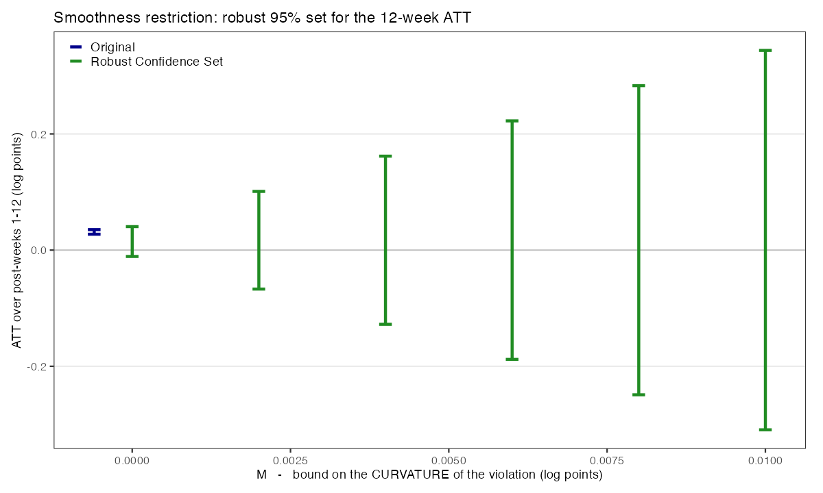
Figure 17.19: `plot(s, type = "sens", restrict = "sm")`, **after the two-line repair below**. The navy **Original** band sits tight above zero at about +3% and **excludes** zero. The very first robust set — at $M = 0$, the *strictest* setting — **already crosses zero**, and the sets fan out from there. That is $M^{*} = 0$, visible.

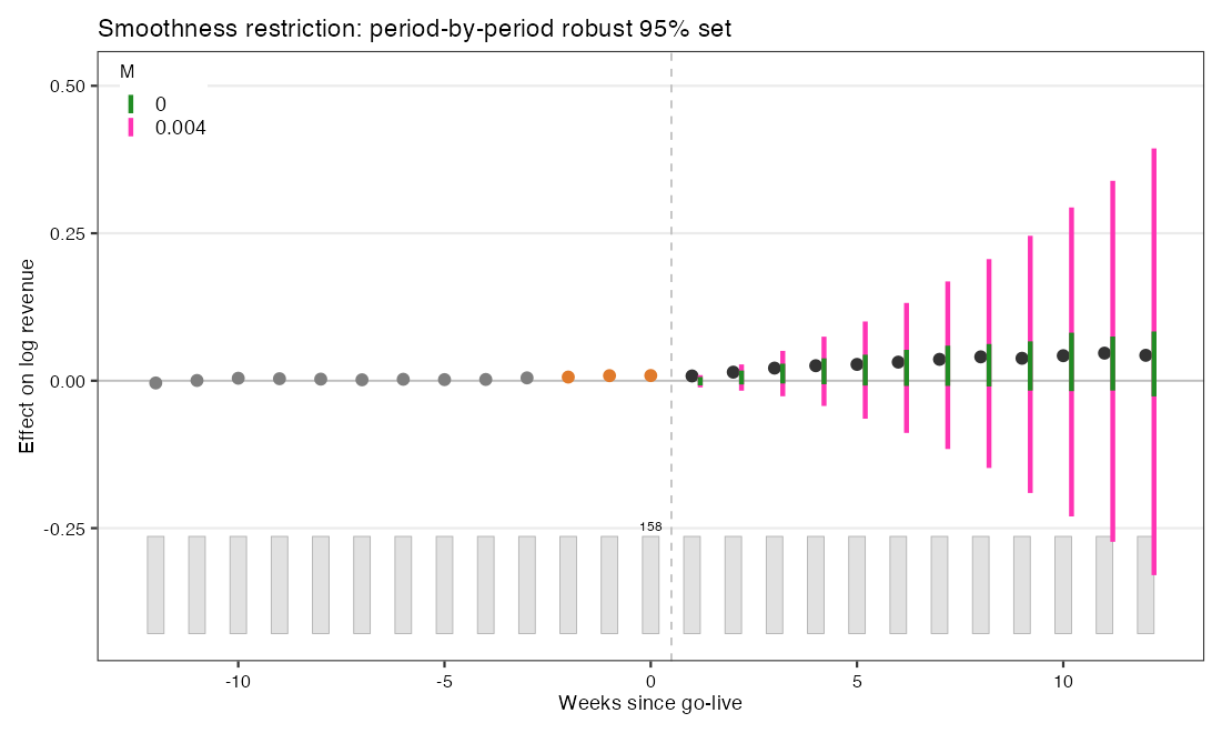
Figure 17.20: `plot(s, type = "sens_es", restrict = "sm")` — the same restriction, period by period. Green is $M = 0$, pink is $M = 0.004$. Every interval contains zero, and both widen sharply with the horizon; by week 12 the pink set spans roughly −33% to +39%.

The picture was broken. The numbers never were. (fect defect, re-diagnosed)

A bare plot(s, type = "sens", restrict = "sm") comes out unreadable: what look like horizontal bars sprayed across the panel, and the “Original” band parked far off to the left. It is tempting — and this course’s notes said so until we actually read the source — to call it “transposed.”

It is not transposed. plot.fect builds aes(x = M) with a vertical geom_errorbar, which is correct. The bug is two constants hardcoded in x-axis units, written for the $\bar M$ scale and reused verbatim for $M$:

where	constant	on $\bar M \in [0,1]$	on $M \in [0, 0.010]$
the errorbar cap width	`width = 0.02`	a 2% tick — fine	200% of the x-range
where Original is parked	`x = -0.05`	just off to the left — fine	5× the domain away

$\bar M$ is unitless — a multiple of a ruler — so it always lands in $[0,1]$ and the constants always work. But $M$ is in the outcome’s own units. On log revenue it spans 0.010, so every errorbar’s cap is wider than the plot. The “horizontal bars” are the caps.

The repair is two lines, and it touches no data:

# (a) plot.fect only defaults Original to x = -0.05 IF the column is missing. Supply it.
s$sensitivity.smooth$original$M <- -6e-4
p <- plot(s, type = "sens", restrict = "sm")
# (b) the cap width should be ~2% of the x-range: 0.02 * 0.010 = 2e-4.
p$layers[[2]]$geom_params$width <- 2e-4
p

That produces Figure 17.19. The numbers in the object were right the whole time — as the table above, read straight off it, already showed.

The lesson is not “distrust the picture”

The identical call renders perfectly if your outcome is in levels (rescale $M$ by 100 and the bare call is fine — no patch at all). So this bug fires for some analysts and not others, purely on a modelling choice that has nothing to do with it. ⚠️ “It worked for me” proves nothing.

That is the real lesson, and it generalises far past fect: a plot that renders is not a plot that is right, and a plot that renders for you is not a plot that is right for anyone else. When a figure and an object disagree, the object is the evidence — go read the source and find out why, because “the package is buggy” is not a diagnosis.

(And the $+4.04\%$ upper bound at $M = 0$ is the same $20\times\text{SE} = 0.0403937$ lid that flattens Figure 17.17 — the smoothness set is censored at the top too. Its lower bound is clean, which is the only reason $M^{*} = 0$ stands. Do not read the upper edge as a bound.)

17.3.5.7 Walk back the dials you turned without being asked

Table 17.10: Four dials, none of them asked for your consent.

the dial	what you set	what it decided
the window	`proportion = 0.3`	whether the pre-trend certified at all (TOST 0.082 → 0.000)
the bar	$\theta = 0.36 \times \sigma_{\text{FEct}}$	what counts as negligible — here 46% of the effect
the restriction	$\Delta^{RM}$, not $\Delta^{SD}$	the violation’s shape — and it flips the verdict from 0.46 to 0
the grid	`by = 0.05`	printed $\bar M^{} = 0.50$; refine it and it is 0.46*

The memo rule — this is what A5 is graded on

Declare the window, the bar, the restriction and the grid before you look at the set. Justify the restriction by the shape you expect the leftover to have — never by which one survives. If you cannot name the shape, report both.

And then the closer, because it is the sentence the whole session has been building: every ruler in this act was cut by the model under test. The band it calls negligible is 0.36 × a different model’s residual SD. The scale $\bar M$ is its own worst pre-period step. The setting called zero is its own last imputation error, frozen. There is no verdict here. There is a price — and a price is not a number until you name its currency.

In estimation, the penalty is the assumption. In inference, the restriction is the assumption.

17.3.5.8 A point needs a band — and the right band depends on the design

“A point estimate without a band is not a finding,” but which band depends on how the study was run — and after the last three subsections, “which band” plainly includes “under which restriction.” Three design choices carry most of the remaining weight (Liu, Wang, and Xu 2024). Cluster at the assignment level: the app was rolled out to markets (40 of them), not individual stores, so the standard errors must cluster on the 40 markets — clustering at the store would treat correlated within-market store-weeks as independent and overstate precision. Match the resampling to the treated count: a nonparametric block-bootstrap over units is the default, but when the number of treated units is small the bootstrap turns unreliable and the jackknife is more stable. Joint, not pointwise, bands for trajectories: an event study’s per-period pointwise CIs jointly under-cover the whole path, so any claim about the entire trajectory needs simultaneous (joint) bands (Cattaneo et al. 2025). And for factor / matrix-completion estimates the interval itself is the provisional part — getting a valid band is a genuine open frontier (inference under not-at-random missingness (Choi and Yuan 2024; Choi, Kwon, and Liao 2024); doubly robust inference in latent-factor models (Abadie et al. 2024); the Part-IV sensitivity discipline carried forward (Bach et al. 2025)) — so report it and flag it. The A5 discipline: name your assignment level, size the resampling to how many treated units you have, never dress a pointwise interval up as a joint claim — and name the restriction behind any robust interval you quote.

17.3.6 Effect heterogeneity

17.3.6.1 The fit returned a matrix, not a number

IFEct did not hand back an effect. It handed back an eff matrix: an estimated effect for every one of the 5,606 treated store-weeks. The +4.78% you have been quoting is one summary of that matrix — the grand mean. It is not privileged; it is simply the first average anyone took.

So the estimator is finished before this section begins, and everything that follows is reading. And the rank stays where cross-validation put it: $r = 1$, fixed. Nothing below is a new estimator; every number is a different average of the same matrix — or a refusal to average at all.

How this differs from Session 09 — say it precisely, because the difference is not the one you would guess. It would be false to claim S09 needed a new estimator per view: S09’s own recap was titled “One Score, Four Jobs,” and GATE, BLP, RATE, CLAN and the policy tree all ran off the same orthogonal score. S09 was already a one-object-many-projections session. The real difference is the object. S09’s $\psi_i$ is a noisy but unbiased score whose conditional mean is $\tau(x)$, so it must be projected to be read — and that projection is testable: BLP regresses $\psi$ on $\hat\tau$ and tests the slope. A cell effect in a factor-imputation model has no orthogonal score. There is no BLP analogue, and therefore no test that the heterogeneity is real — only a refusal, and then an aggregation. That is the whole shape of this section.

17.3.6.2 Lens 1 — same fit, two axes, two illusions

Do not aggregate at all. plot(f, type = "box", xlim = c(1, 12)) shows every treated cell, week by week (Figure 17.21). The picture is alarming: of 1,896 treated store-weeks in the first twelve weeks, 21.4% read NEGATIVE (sd 3.71 pp) — and in week 1 alone, 38.6% do. Four seconds is all an executive needs: pull the app from the losers.

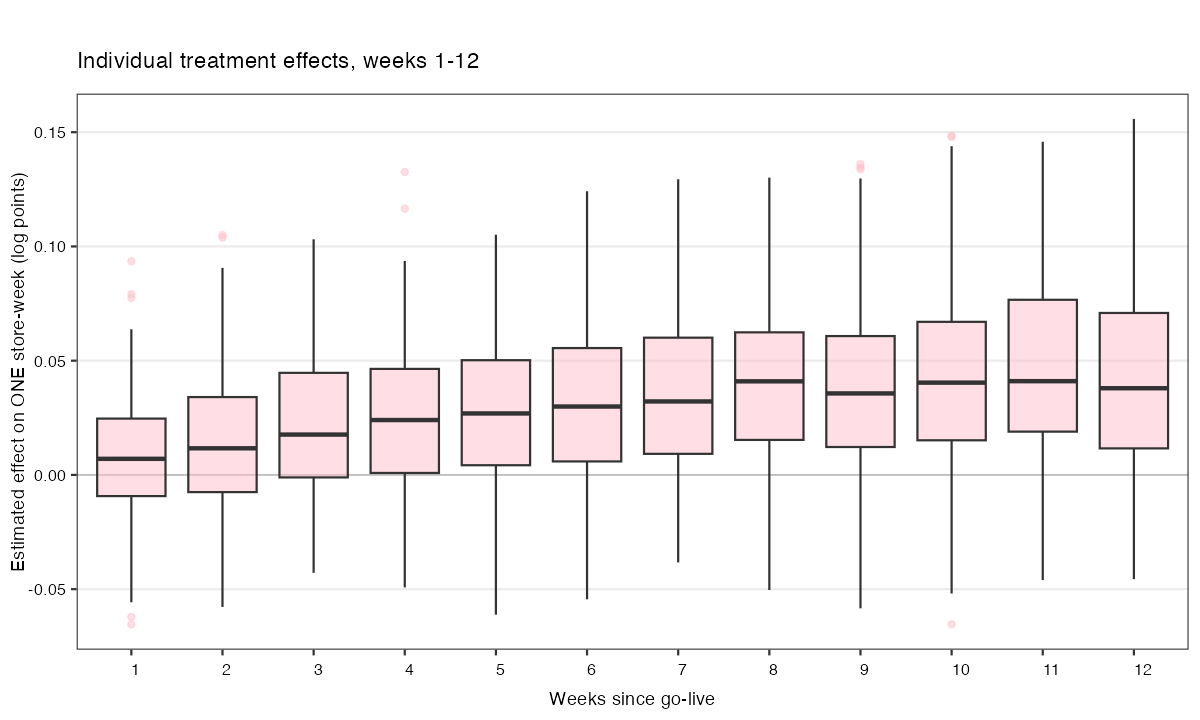
Figure 17.21: `plot(f, type = "box", xlim = c(1, 12))` — the estimated effect on every individual treated store-week, weeks 1–12. 1,896 cells; 21.4% of them sit below zero, and 38.6% do in the launch week.

Now change one argument. Same call, same fit: xlim = c(-12, 12) (Figure 17.22). The new blue boxes are the same 158 stores in the thirteen weeks (event time $-12 \ldots 0$) before their own go-live — cells where no app exists and the effect is zero by definition. (Note fect’s axis convention once and it saves you later: event time 1 is the launch week; 0 is the last pre week.)

48.0% of those cells read NEGATIVE. Not 0%. Forty-eight.

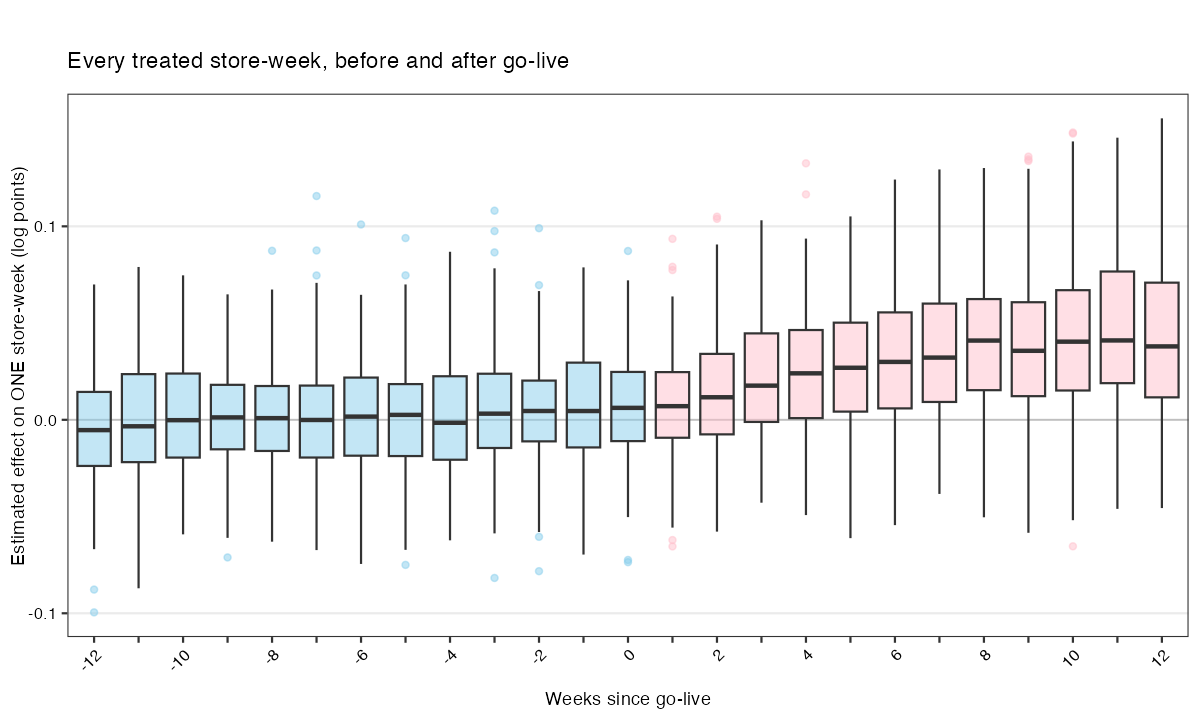
Figure 17.22: The identical call with `xlim = c(-12, 12)`. The pre-launch boxes are the same 158 stores in the thirteen weeks before go-live — a window in which nothing happened. 2,054 cells, **48.0% negative**, sd 2.97 pp. Compare like with like — one box against one box: the *null* box (week 0, IQR **3.58 pp**) is **taller** than the *signal* box (week 1, IQR **3.39 pp**).

The null value of ‘% of cells reading negative’ is 50, not 0

Say this precisely, because the sloppy version is wrong and a sharp student will kill it. The claim is not “the model thinks half the stores were harmed.” The claim is that the null value of the statistic is 50.

Why 50? Because treatment is absorbing. A treated store’s only untreated cells are its pre-launch cells — and that store’s unit fixed effect is fitted on exactly those cells. The normal equations therefore force its pre-period residuals to average exactly zero. Half of them land below. That is an algebraic identity, not a finding about coffee.

And notice what the argument did not need. It did not claim the true pre-window effect is zero — and it must not, because this session has already shown it cannot certify that: the placebo fired at +0.78 pp, and TOST could not certify the pre-window as small (0.082). The identity holds whatever the true pre-effect is. That is why this argument is airtight and the seductive one is not.

So “21% read negative” is 21 measured against a null of 50, not against 0 — a signal-to-noise ratio wearing a harm rate’s clothes. And read the boxes, not the shares — comparing like with like, one box against one box: the last pre week (week 0, IQR 3.58 pp) against the first post week (week 1, IQR 3.39 pp), the exact moment the pull-the-app call gets made. The null box is taller than the signal box. At launch the signal is not merely small relative to the noise; it is indistinguishable from it. (Pooling all 2,054 pre cells gives an IQR of 3.94 pp, but that number is inflated by between-week variation — do not set it against a single week’s box.)

Is the 50% a property of IFEct, or a property of imputation? Run four imputers of wildly different quality on the same panel and count (Lab 4 does this live):

Table 17.11: The ~50% is a normal-equations identity, not a modelling result. Every imputer returns it.

imputer	% negative, full pre-window	% negative, last 12 pre-weeks
unit FE only	51.2%	34.0%
two-way FE	50.2%	48.5%
IFE $r=1$ (our fit)	50.2%	48.0%
IFE $r=4$ (deliberately over-fitted)	50.2%	49.8%

Be honest about the second column, because it is where the identity is only approximate. Over the full pre-window the identity is exact — the unit FE is fitted on precisely those cells. On the last-12 window (the sub-window the figure draws), an imputer that does not absorb the common time trend — unit-FE-only — drifts to ~34%, because the late pre-weeks sit above the store’s own pre-mean. Every model you would actually use absorbs the trend and lands at 48–50%.

A prohibition on reading a cell — not a denial that heterogeneity exists

This is the scoping sentence, and it is not optional. Nothing above says heterogeneity is absent. In three subsections we will split these same stores three ways and find a 5.75-point spread with standard errors of a fifth of a point. Heterogeneity is real. Cells are not readable. Both are true, and only aggregation buys the difference — which is exactly Holland’s fundamental problem of causal inference, as a number: an individual treatment effect is not identified by any estimator, however good.

And say the prohibition both ways, because someone will try to rescue the tails: the same imputation error that invented harm here would just as happily hide real harm if it existed. You cannot read the tails for good news either.

So how should you read Figure 17.22? A refusal is not a reading. Read the location of the distribution — not any one box, not the share negative, not the width. In the pre-window the median sits at zero, as it must. After launch it lifts, and keeps lifting: +0.7% in the launch week, +4.1% by week 8. That climb is the effect — it is precisely the ramp the event study reports, arriving one week at a time. The figure is not useless; you were reading the wrong feature of it.

And you cannot rescue heterogeneity from the width, either

The natural next move is: “fine — then the spread is the heterogeneity. The post boxes are visibly fatter, so stores must differ.” They are fatter — and it is not heterogeneity.

Post IQR grows from 3.39 pp (week 1) to 5.93 pp (week 12), and that widening is imputation error growing with the horizon: post cells are out-of-sample extrapolations, and the further you extrapolate the worse you predict.

Worse, the pre boxes understate the noise floor. Those residuals are in-sample — the unit FE is fitted on exactly them, so they are shrunk toward zero. The pre spread is therefore only a lower bound on the imputation error.

⇒ You cannot subtract the variances and call the remainder heterogeneity. Not the level, not the tails, not the spread. The only thing this figure licenses is the location. (Real heterogeneity does exist here — Lens 3 finds a 5.75-point spread with SEs of a fifth of a point. It takes an aggregation to see it, never a cell.)

17.3.6.2.1 The same fit on a different axis — and the second illusion

The cell is unreadable, so aggregate. That is what aggregation is for. And ask the most natural managerial question there is: does the app work better at some times than at others? Season, macro conditions, a competitor’s response, word-of-mouth compounding across the year. One argument: plot(f, type = "calendar") (Figure 17.23).

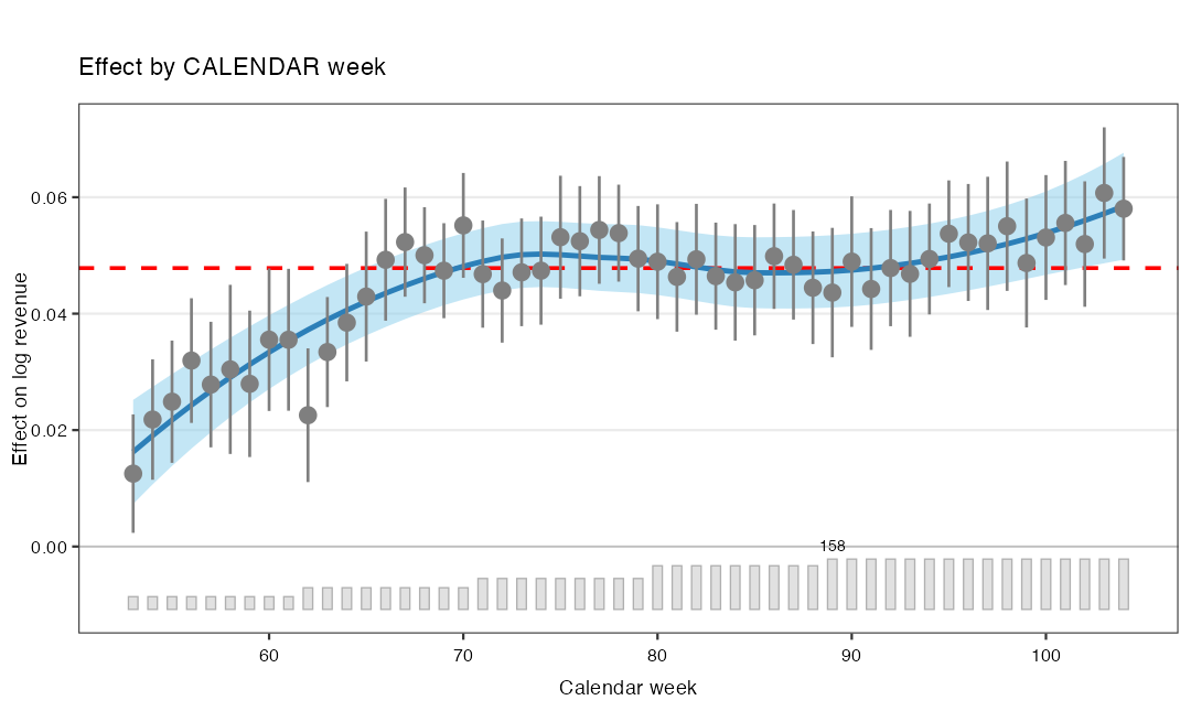
Figure 17.23: `plot(f, type = "calendar")` — the ATT by **calendar** week, same fit as Figure 17.22. It climbs from **+1.25%** in week 53 (CI [+0.23, +2.27]) to **+5.80%** in week 104 (CI [+4.91, +6.69]); the red dashed line is this fit’s own ATT, **+4.78%**. The grey bars are the treated count — 40 stores, then 68, 97, 137, 158, as the five waves go live.

The path climbs from +1.25% to +5.80% — a 4.8-point swing, as large as the entire ATT. Every instinct in the room says the same thing: the app is getting better over time. Network effects. Word of mouth. It compounds.

There is no calendar in the calendar plot

Look at the grey count bars, which fect draws for you. In calendar week 53 the treated set is 40 stores, every one of them in its first week of tenure. By week 104 it is 158 stores at a mean tenure of 35 weeks. And this effect ramps with tenure — read it off the very same fit: +0.8% in event week 1, +4.3% by week 12.

So the calendar path is not measuring calendar. It is measuring the ramp, sampled through a staggered rollout: at every calendar week the treated set is a different mixture of tenures, and the mixture matures as the rollout completes.

The proof is checkable, and it uses no oracle. Take the event-time ramp — one number per tenure, nothing else — and average it over whichever tenures happen to be treated in each calendar week. There is no calendar term anywhere in that calculation. It reproduces the observed path inside the estimate’s own 95% confidence interval in 48 of the 52 weeks (mean gap 0.52 pp against a mean standard error of 0.52 pp — the reconstruction sits inside the noise). A model that does not know what a calendar is draws this curve.

And the dips prove it twice. At weeks 62 and 71 the curve drops 1.30 and 0.84 points, and each drop lands exactly on a go-live wave: 28 new stores, then 29, each entering at tenure 1 with almost no effect yet, dragging the average down. The rollout dilutes its own average. (Waves 4 and 5, at weeks 80 and 89, barely dent it — 0.05 and 0.08 pp — because by then they are a small addition to a large, mature treated base. Do not oversell a sawtooth that is only visible twice.)

Now be fair to the plot: same numbers, two estimands

“No calendar in it” is a statement about one estimand, not a verdict on the figure — and a good student will defend it, correctly. Figure 17.23 is the right answer to a genuinely different and genuinely managerial question:

What did the app actually deliver, week by week, across the fleet that was live at the time?

That number really was +1.25% in week 53 and +5.80% in week 104. Nothing there is an artifact. If the CFO asks how much revenue the app added in Q4, this is the right plot and the event study is the wrong one — and the late figure is high precisely because the fleet was mature, which is a fact about the business, not a bias.

So state it exactly. Same numbers, two estimands. Read as delivery, the curve is true. Read as effect modification by calendar time — “does the app work better in some weeks?” — it is empty, because a reconstruction carrying no calendar term reproduces it. And nothing on the face of the plot tells you which one you asked. That is why the lesson is “the axis is the question,” not “this plot is junk.”

A trace note, because a sharp student will catch it — and it is the lesson in miniature. The red dashed line in Figure 17.23 is +4.78%, not the +4.76% headline. Both are correct: +4.76% belongs to the CV-selected fit, while Figure 17.23 is drawn from the fixed-$r$ refit, and the line it draws is that object’s own ATT. The ramp endpoints move the same way (+0.75% / +4.25% on the CV-selected fit, +0.76% / +4.28% here). A number is a property of a fit, not of a session — always re-derive it from the object the figure actually calls, never by copying it off another slide.

You have just diagnosed the bad control you meet three pages from now

Hold on to “calendar week is confounded with tenure in a staggered absorbing rollout.” In Section 17.3.6’s second lens, fect will cheerfully draw you a CATT curve against temp_c — weather, a covariate the treatment demonstrably does not move ($p = 0.21$). Its sin is not endogeneity. Its sin is that 95% of temp_c’s level is the calendar week (on the treated cells the plot uses) — so its x-axis is the axis you have just watched lie. Same confound, second costume.

So the two lenses land the same blade from opposite sides. The cell said one in five is hurt, and the null of that statistic was 50. The calendar said the effect doubles across the year, and it had no calendar in it. Neither number is wrong. Both readings are — and the error is not in the data. It is in what you aggregated over and what you plotted against. The aggregation is the question, which is the blade of S09 and the one A5 is graded on.

17.3.6.3 Lens 2 — Route 1: `group=` — split the panel, and let `fect` refit

The moderator you actually want is urban_share, and it is a store attribute: constant in time. Put it in the outcome model and the unit fixed effect absorbs it entirely — there is nothing left for a coefficient to identify. fect does not fail quietly; it refuses at fit time and names your variable:

Error in fect.default(...) :
  Variable "urban_share" is unit-invariant. Try to remove it.

It refuses all six BeanBuzz store attributes this way — urban_share, market_size, seats, drive_thru, baseline_tier, competitor_density — because the within-store standard deviation of every one of them is exactly 0. That is every moderator a manager actually cares about.

But group= never puts the covariate in the model at all — it splits the panel. A discrete split has no slope, so there is nothing for the unit fixed effect to eat. fect refits the whole estimator inside each group and bootstraps each one. The constraint evaporates — not through cleverness, but because you asked a different question.

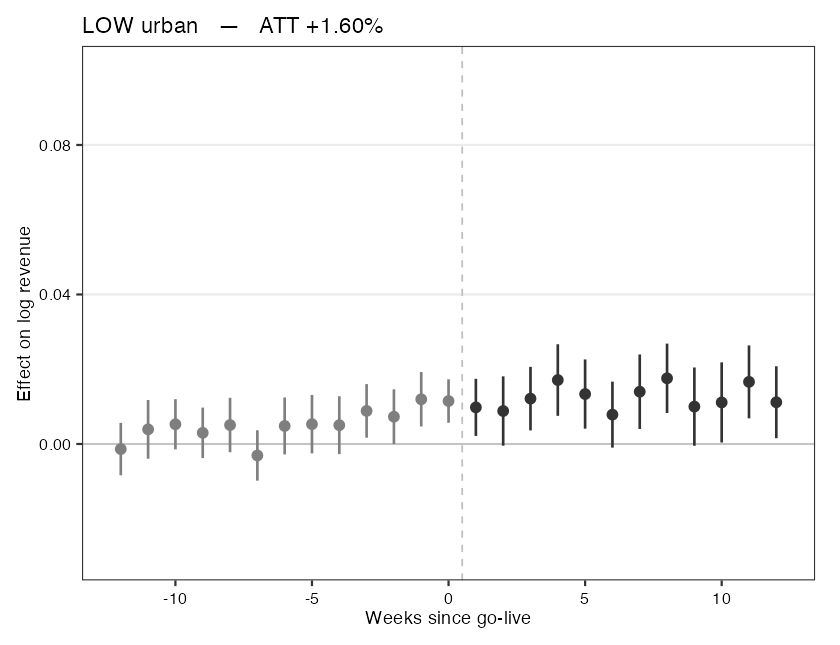
Figure 17.24: `plot(fg, type = "gap", show.group = "Low urban")` — **ATT +1.60%**. Flat: the ramp barely leaves zero.

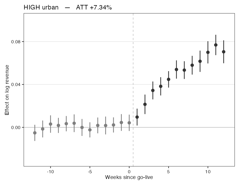
Figure 17.25: The same call, `show.group = "High urban"` — **ATT +7.34%**. The ramp climbs to ~+7%.

Pin the y-axis, or the picture will contradict the numbers

fect auto-scales each group’s panel to its own data. Draw Figure 17.24 and Figure 17.25 with the default limits and Low urban (+1.60%) and High urban (+7.34%) render as visually identical ramps on different axes — the pair would say “no heterogeneity” while the table screamed the opposite. Both figures above are pinned to a common ylim. The heterogeneity is the gap between the panels, and you only see a gap if the panels share a ruler.

The call is one argument:

fg <- fect(log_rev ~ app_live, ..., group = "urban_tertile")
fg$est.group.att

Table 17.12: A 5.75-point spread under a +4.78% average, and the intervals do not touch. Heterogeneity is real — this is the aggregation that buys back what the box forbade.

`fg$est.group.att`	ATT	S.E.
Low urban	+1.60%	0.21 pp
Mid urban	+4.61%	0.21 pp
High urban	+7.34%	0.21 pp

Read the row names, or you will brief the board on the wrong stores

Print fg$est.group.att, never fg$group.att. The latter is an unnamed vector, and if you assume it runs low → mid → high you will tell a board to abandon the wrong stores. And even the named matrix prints alphabetically — High, Low, Mid — not in tertile order. Read the row names.

Now catch it with your own rule. est.group.att averages every post cell it has. The effect ramps with tenure. And the low-urban stores went live about nine weeks later than the rest — mean treated tenure 18.8 / 26.2 / 27.9 weeks for Low / Mid / High. So the three groups are being averaged over windows of different lengths on a growing path. That is composition, and it is the trap this course has been drilling since S10.

Put all three on a common 12-week horizon:

Table 17.13: 36% of the headline moderation is rollout timing on a ramping effect. The moderation survives; the number does not.

group	ATT, all post weeks	ATT, common 12-week horizon	mean treated tenure
Low urban	+1.60%	+1.25%	18.8 wk
Mid urban	+4.61%	+2.92%	26.2 wk
High urban	+7.34%	+4.94%	27.9 wk
spread	5.75 pp	3.69 pp

The three common-horizon effects average to +3.04% — the same object the sensitivity act bounded. Part V has one estimand, not four. And note precisely how this differs from S10: S10’s staggered TWFE gave you a wrong number. This gives you an honest average of a different estimand — which is worse, because the arithmetic is correct, the question has quietly changed, and nothing warns you. (Point estimates only: fect prints no interval for a windowed group ATT. Do not hand-roll one.)

Now audit it. One flag: group= and placeboTest = TRUE together. Blank the last three pre-weeks and re-impute them out of sample inside each group, then ask the only question available without an answer key: does the moderation show up in cells where the effect is zero by design?

fpg <- fect(log_rev ~ app_live, ..., group = "urban_tertile",
            placeboTest = TRUE, placebo.period = c(-2, 0))
plot(fpg, type = "gap", show.group = "Low urban")   # prints TWO p-values

Table 17.14: A placebo inside each group. Both p-values are printed on the figure — the per-group equivalence p exists nowhere else in the object.

group	ATT	placebo	placebo $p$	placebo-equivalence $p$	verdict
Low urban	+1.60%	+1.29 pp	0.000	0.348	cannot certify
Mid urban	+4.61%	+0.43 pp	0.330	0.011	certified
High urban	+7.34%	+0.58 pp	0.134	0.014	certified

Low urban’s placebo is 81% of its own headline effect. On Figure 17.26 its orange placebo triangles sit at the same height as its early post-launch points; on Figure 17.27 they sit on zero.

The one group a board would deprioritise is the one group whose number it cannot use.

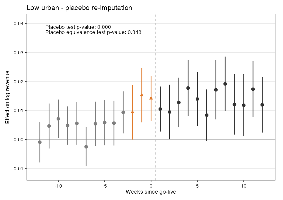
Figure 17.26: `plot(fpg, type = "gap", show.group = "Low urban")`. The blanked placebo cells come back at +1.29 pp — 81% of this group’s own +1.60% headline effect. Placebo p = 0.000; placebo-equivalence p = 0.348, so the violation **cannot be certified as small**.

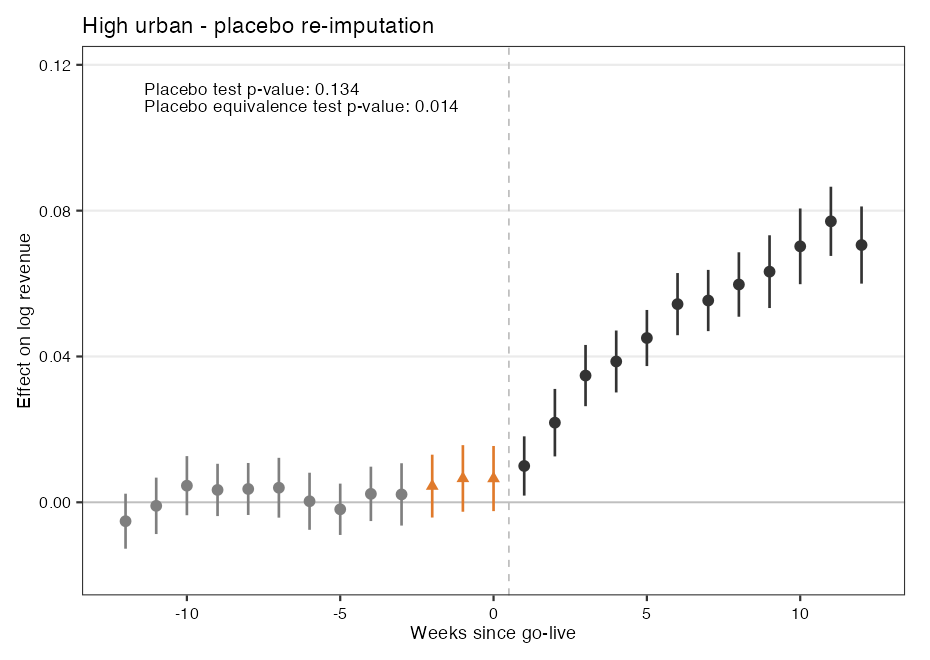
Figure 17.27: The same call, `show.group = "High urban"`. The placebo cells sit on zero (+0.58 pp, p = 0.134), and the equivalence test **affirms smallness** at p = 0.014.

The audit can CONVICT. It cannot ACQUIT.

Do not say “High urban passed because $p > 0.05$.” That is absence of evidence, and we spent an entire act on it. High urban passed because the equivalence test affirmed smallness (0.014). That is the whole difference, and it is the third time Part V has made you meet it.

The audit convicts Low urban. Now say the three things it does not license — because each is a sentence you will want to write, and none of them is available:

Not “the error is group-differential.” Low minus High is about +0.71 pp with SE ≈ 0.54 — the data cannot reject that all three groups carry the same bias. Inferring a difference from “one p is significant and the others are not” is exactly the fallacy this section exists to police.
Not “subtract each placebo from its own ATT.” That is not $\bar M = 0$, it is not any restriction in the HonestDiD menu, and it is precisely the frozen-level move the sensitivity act refused.
Not “the ranking is safe.”

And here is why the beautiful standard errors did not save you. The bootstrap prices sampling noise, not a wrong counterfactual. Those 0.21-pp SEs are perfectly honest about how much a group ATT would move if you re-drew the stores. They are completely silent about whether $\hat Y(0)$ is the right counterfactual. That is what the placebo is for — the only instrument in this section allowed to say no.

17.3.6.4 Lens 3 — Route 2: `type="hte"` — four hurdles, and you must build the covariate

group= gave you three rungs. plot(type = "hte") promises a continuous curve — and everyone reaches for it first. It is worth knowing exactly what it costs.

What the plot actually does, because it is not what people assume: it takes the cell effects, takes the covariate’s raw level at each of those cells, and loess-smooths one against the other. That is all. It is a kernel-weighted group= with a continuous axis. And it demands the covariate be in the outcome model — which imposes four hurdles.

Table 17.15: The four hurdles. No raw covariate in the BeanBuzz panel clears all four.

the covariate must…	or else — and what it kills
1. vary within store	the unit FE eats it → “unit-invariant”. Kills all 6 store attributes, `urban_share` included
*2. be nonzero on the untreated* cells**	`fect` fits $Y(0)$ only there. `urban_share × app_live` is identically 0 → collinear with the FE. The moderator is only “on” where `fect` refuses to look.
3. not be moved by the treatment	else it is a bad control. Kills `mktg_spend`: +€251, t = 130
4. not be a clock	else you are plotting the tenure ramp in disguise. Kills `temp_c` (95% week) and `footfall_index` (88%)

Hurdle 2 is the deep one: the moderator lives inside the block fect refuses to look at

The obvious fix to hurdle 1 is “fine — make it time-varying: interact it with the treatment.”

df$urban_x_app <- df$urban_share * df$app_live      # varies within store now
fect(log_rev ~ app_live + urban_x_app, ...)
#> Error: The only variable, 'x.1', is collinear with the fixed effects.

It cannot work, and the reason is the whole imputation idea. fect fits the $Y(0)$ model on the observed — i.e. untreated — cells only: fit the white cells, predict the grey ones. And urban_share × app_live is identically zero on every untreated cell (sd = 0.000000). The regressor is invisible to the fit and collinear with the fixed effects.

A treatment-effect moderator is, by construction, only “on” inside the very block fect is trying to predict. You cannot teach the imputation model about the moderator using the cells it has sworn off.

The API’s constraint selects for BAD CONTROLS

Hurdles 1–4 together are not bad luck; they are structural. The covariates fect will draw a curve for are exactly the time-varying ones — and in an absorbing rollout, the time-varying ones are exactly the ones your treatment may have moved (mktg_spend: +€251, t = 130, and it moved the headline too, +4.78% → +4.82%), or the ones that are secretly a clock (temp_c is 95% calendar week; footfall_index 88%).

And note the asymmetry, because it is Session 02 arriving for the last time: the treatment test convicted mktg_spend and acquitted temp_c (p = 0.21) — and temp_c is still unusable. The treatment test is necessary and never sufficient. The data will never clear a control. Only the graph can.

Never read a package’s willingness to draw a plot as a licence to interpret it.

So build a covariate that clears all four.

df$urban_x_week <- df$urban_share * df$week

fuw <- fect(log_rev ~ app_live + urban_x_week, data = df,
            index = c("sid", "week"), method = "ife", r = 1,
            force = "two-way", se = TRUE)

plot(fuw, type = "hte", covariate = "urban_x_week")

Check it against each hurdle, and the fourth one is the surprise:

within-store sd 15.8 → fect accepts it.
sd 17.5 on the untreated cells → fect can actually fit it. This is exactly where the app_live interaction died.
It is deterministic in (store, week), so the treatment cannot move it. Hurdle 3 is not passed — it is unpassable by construction.
On the treated cells — the only cells this plot uses — it is 88% store trait and 5% calendar. Why? Because among treated cells the calendar spans weeks 53–104 (a factor of 2) while urban_share spans 0.1–0.9 (a factor of 9). The product is urbanity, not time.

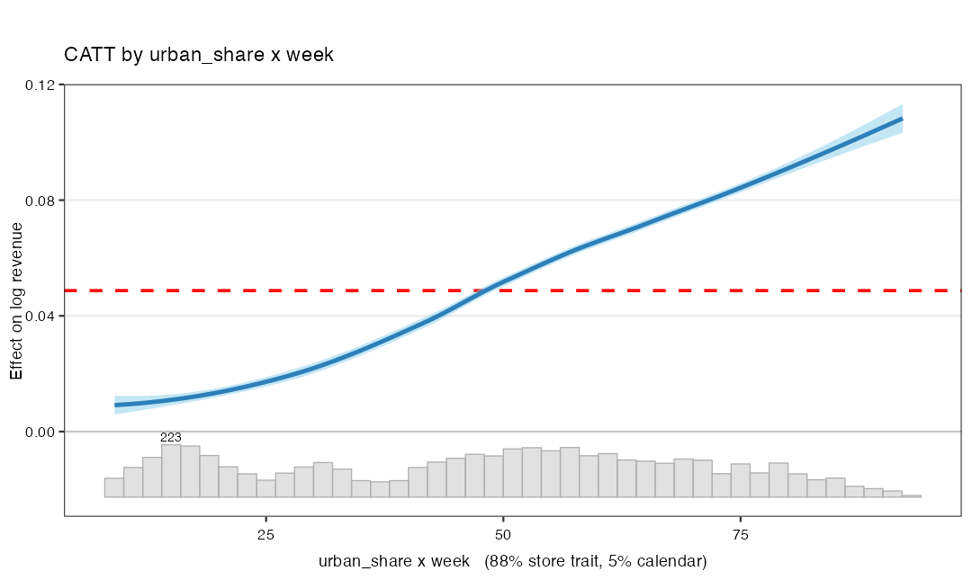
Figure 17.28: `plot(fuw, type = "hte", covariate = "urban_x_week")` — the CATT smoothed against the constructed moderator. It sweeps **+0.9% → +10.8%**, monotone, and it **agrees with the tertiles** of Table 17.12. The red dashed line is this fit’s own ATT (+4.87%).

Two prices — and the second one is the reason group= exists

The curve is a continuous gradient where group= gave you three rungs, and it agrees with them. That payoff is real. It is not free.

Price 1 — the covariate is in the model, so it moved the estimator. +4.78% → +4.87%. group= never touches the estimator; it only splits the sample. You bought a nicer picture with a different headline.

Price 2 — that ribbon is not an inference band. Read the source: it is qt(0.975, df) × loess se.fit, computed over the 5,606 cell effects treated as independent observations. It does not propagate the imputation uncertainty. It does not cluster by store or market. And — the part that surprises everyone — it never touches the bootstrap, even on this fit, where se = TRUE and 200 bootstrap draws are sitting in the object. It ignores them. A tight ribbon here means nothing except “loess had a lot of points.”

⇒ group= gives you a BAND. type="hte" gives you a SHAPE. Use the shape to see the gradient; use the band to defend it.

17.3.6.5 The close: two headline ATTs, and the estimator picks neither

print(f) — the first thing you ever typed in this session — hands you two headline ATTs and picks neither:

+4.78% weighting store-weeks equally (SE 0.25 pp)
+4.41% weighting stores equally (SE 0.26 pp)

And here is the part nobody tells you: every figure in this section — the boxes, the gap plots, the group panels, the reference lines — silently used the cell convention. If your board cares about stores, not store-weeks, then not one figure you have seen is the one they want, and nothing warned you.

The aggregation is the QUESTION

The penalty was the assumption. The restriction was the assumption. And then the estimator stops.

Which average you quote is not an assumption — it is the question, and no package will ever answer it for you.

17.3.7 The bake-off and the board memo

17.3.7.1 The board wants one number, defended

We now have a ladder of estimates for the identical grey block — from the naive +16.3% (off the ladder, pure selection) down through the additive family to the factor family near +4.9% (Figure 17.12). To an analyst that ladder is fascinating; to a board it is noise. A board runs a decision — launch wider, hold, kill — and a decision needs one number, a band around it, and a defensible reason for choosing the estimator that produced it. The reason cannot be “it was the biggest” or “it had the tightest interval” — per Section 17.3.2 it must be “its assumption is the most credible one for this panel.” This section is the A5 rehearsal — kept off the lecture slides and worked as the take-home after Lab 4: run the bake-off, then write the memo. (It is deliberately outside the PBL block: the memo is writing rather than coding, and A5’s Part H grades the bake-off and board memo for real, at 7% of the assignment.)

17.3.7.2 Read it as a ladder, ranked by assumption credibility

A forest plot invites two wrong readings. Wrong reading one: average the eight numbers — absurd, because they encode different and contradictory assumptions, and averaging a credible estimator with a discredited one just contaminates the credible one. Wrong reading two: pick the tightest confidence interval — also wrong, because tightness reflects the model’s confidence in its own (possibly false) assumption, not its correctness; the naive estimator can be precisely wrong. The right reading treats the forest as a ladder ordered by assumption richness and asks, at each rung, is this assumption defensible for this panel?

Naive +16.3% — the lone outlier. Ignores the design entirely; selection, not effect. Discard.
Additive family (CS / TWFE / imputation, ~+3.3–4.2%) — honest but blind to the latent wave; biased down. Trust the floor, not the level.
Factor family (IFEct +4.8%; MC +4.3% under-recovers) — sees the dominant latent wave; IFEct lands on truth. Most defensible here — because regional economic cycles (and, more faintly, seasonality) plainly move coffee retail. (But MC is a low-rank tool that under-recovered, not a second “factor family” member to average with.)

You do not average a ladder. You climb to the rung whose assumption you can defend — and here that rung is the factor model, not because it is biggest or tightest, but because its assumption survives scrutiny in this business context.

17.3.7.3 The 4-sentence board memo

The deliverable of real causal work is not the forest plot; it is the one-line justification plus the band. Build it natively, four sentences, each doing one job:

BeanBuzz loyalty app — recommendation

The number. The app lifted weekly revenue by ≈ +4.8% (band roughly +4% to +5%) across treated stores.
The estimator & why. We trust the interactive-FE estimate: regional economies swing together and stores ride those swings by different amounts (with coffee seasonality a fainter second wave) — latent structure the simpler additive models provably miss (they read +4.2%, biased low). The choice is by assumption credibility, not by the number being convenient.
The key threat. An omitted second factor (a promo cycle, a competitor entry) or selection in which stores launched first could still move the number; the band, not the point, is the finding.
The call. The lift clears the rollout hurdle: proceed to the next wave, instrumented to re-estimate as data accrue.

This skeleton — number, estimator-and-why, threat, call — is the A5 rubric for the write-up portion. Fill these four with your scenario’s specifics and you have the memo. The discipline is brevity plus defensibility: a board reads four sentences, not eight numbers.

17.3.7.4 Your A5 tell: which lens does the estimand demand?

A5 is NOT a BeanBuzz clone

A5 asks about a grocery chain’s self-checkout rollout → footfall, and it carries two estimands, not one. A single flagship market went live alone, with no comparable cohort: start from the estimand — how many treated units? — and one routes to synthetic control (S11), not the interactive-FE-on-a-big-cohort pipeline you just saw built on the 158-treated-store BeanBuzz panel, because for the flagship there is no cohort to average and too little treated signal for a factor model. A handful of later pilots went live on a staggered schedule — those are a genuine many-unit problem and route to the staggered-DiD / imputation pipeline (S10), diagnosed cohort-by-cohort for parallel trends. The trap is not “using a big-cohort method at all”; it is cloning the last technique you saw onto the wrong estimand, or blending the two effects into one headline. Re-derive each question from its estimand; do not reach for the last technique you saw. The underlying logic is identical — it is all imputing the same grey block under one optimization — but the credible rung depends on the data structure: a single flagship demands the synthetic-control rung with a prediction band and a placebo test, while the staggered pilots demand the heterogeneity-robust DiD rung with a per-cohort pre-trend check.

17.3.8 The part closes

Part V was one long project to fill the same greyed $Y(0)$ block under escalating assumptions — S10’s additive parallel trends, S11’s convex donor blend, S12’s low-rank factor — each solving the one optimization of Equation 17.1 under a richer regularizer. The close is deliberately short: the completed assumption ledger, which is the A5 rubric.

17.3.8.1 The field’s verdict: robust DiD kills significance, not signs

Calibrate against the published record before trusting any single headline. Chiu, Lan, Liu and Xu re-ran 49 replicable TWFE difference-in-differences studies with the modern HTE-robust estimators (Chiu et al. 2026). The reassuring half: switching estimators rarely changes a finding’s direction — only 3 of 49 flip sign, just 1 significantly, and the median standard-error ratio is a modest 1.08. The sobering half: what robust methods do change is significance. The share of studies that can no longer reject the null of no effect climbs from 2% under TWFE to 24% under imputation; 25–27% fail their own placebo or pre-trend F-tests; and under Rambachan–Roth sensitivity at $\bar{M}=0.5$, 81% of the 42 well-powered studies can no longer reject (Rambachan and Roth 2023). The lesson for A5 and for practice: the danger in real DiD work is almost never a reversed sign — it is that the finding was underpowered or its parallel trends were shaky, and the robust methods expose it. Robust DiD is honest, and honesty is expensive — it costs significance, not sign.

17.3.8.2 Underneath every rung: strict exogeneity — and the completed ledger

One assumption sits beneath all of Part V, quietly licensing every estimator: strict exogeneity — treatment was not set by the outcome’s own past. This is the feedback gate that licenses every Part-V estimator, and unpacked it forbids four things (Liu, Wang, and Xu 2024; Imai and Kim 2019): no feedback (a revenue dip did not trigger the rollout), no lagged-outcome dependence, no carryover, and no time-varying confounder the treatment itself moves. In BeanBuzz the waves were scheduled at baseline on market size, not in response to revenue, so strict exogeneity is plausible; had managers launched precisely where revenue had just dipped, every number in Part V would be biased, because the “clean” pre-period would itself be a consequence of the treatment decision. That completes the assumption ledger the part has accumulated:

Table 17.16: The Part-V assumption ledger, complete — each rung buys a counterfactual and pays with an assumption you must defend.

Row	Assumption	Buys	Costs
0	Strict exogeneity	licenses all of Part V	no feedback / LDV / carryover
1 · S10	Parallel trends	cheap, additive, whole cohort	blind to a unit×time factor
2 · S11	Hull + loadings	a counterfactual at $N=1$	hull, non-overfit fit, weak inference
3 · S12	Low rank	recovers the latent factor	rank tuning; restriction choice; bands are frontier

If strict exogeneity genuinely fails — treatment responds to past outcomes — you have left the parallel-trends world entirely and need the g-methods family (marginal structural models, PanelMatch), a different course (Chiu et al. 2026).

17.3.8.3 The estimand chooses the lens, not taste

The methods are not interchangeable options chosen by taste; the data structure dictates the method, and A5 grades exactly this judgment. Two questions from the ledger come first: was treatment set by past outcomes? — if yes, strict exogeneity fails and all of Part V breaks (you need g-methods); and does treatment switch off or reverse? — if yes, reach for reversal-robust estimators (fect handles this natively). Once those clear, the estimand picks the rung: one or a few treated units (a single flagship) → synthetic control (S11), because DiD has no cohort to average and a factor model has too little treated signal; many with no suspected factor → DiD / parallel trends (S10); many with a latent factor or cycle → interactive fixed effects or matrix completion (today); rich covariates but no useful time structure → unconfoundedness / matching (Part III). This is the judgment A5 grades — students are handed a business scenario and asked to justify their estimator from the estimand, not to report the number (Arkhangelsky and Imbens 2024).

17.3.8.4 What you can now do

Name the move: see any causal panel number as an imputation of the blanked $Y(0)$ block — the counterfactual is missing data.
Work the dial: place FEct / IFEct / MC on the one-objective map as one nested regularization dial (additive $r=0$ → hard-impute rank $r$ → soft-impute nuclear norm), and state each one’s assumption as a business sentence.
Prove DiD is imputation: show FEct = BJS = hand-rolled = +4.2% to the digit, in R and Python — the dial at $r=0$.
Recover the factor: use interactive FE to see the omitted latent wave (+4.2% → +4.8% → true +4.9%) — and know that more flexible $\neq$ more right (MC +4.31%).
Stress-test it with no answer key (four tests, four nulls, no verdict): ask for the third pre-trend p-value fect hides — then know that an in-sample pre-trend is the model grading its own homework, because leave-one-out sends TOST 0.082 → 0.350 and nothing certifies; know that the window, the bar ($\theta = 0.36\times$ a different model’s residual SD) and the grid were all chosen for you; read a placebo as a ruler (0.240 pp — a step), not a gate; report the breakdown as a pair ($\bar M^{*}=0.46$ = 0.11 pp/week); treat every fect_sens upper bound as censored until checked against $20\times\text{SE}$; never compare a bare $\bar M^{*}$ across models — and know that the same fit, same panel, same estimand dies at $M^{*}=0$ under smoothness: the restriction is the assumption.
Refuse to read a cell, then aggregate: know that the null value of “% of store-weeks reading negative” is 50, not 0 (a normal-equations identity); that the API’s constraint selects for bad controls; and that a group= split (+7.3% / +4.6% / +1.6%) must be caught on composition and audited with a placebo that can convict but never acquit.
Decide: run a bake-off and write a 4-sentence board memo that picks one estimator by assumption credibility and reports a band.

17.3.8.5 Pointers beyond today

Signposts, not detours — each pushes the imputation idea further; for the curious, not exam material:

Deep-learning imputation — SyNBEATS adapts the N-BEATS neural forecasting architecture to predict the $Y(0)$ cells, often matching or beating SC / TWFE / SDID / MC on benchmark cases (the California tobacco tax, German reunification) (Goldin, Nyarko, and Young 2024). “Impute the grey cells” is method-agnostic: once you see the move, you can plug in any predictor, including a neural net, as long as the design is settled.
Nuclear-norm / SVD theory — the linear algebra under matrix completion: recovering a low-rank matrix from a sparse, non-randomly-sampled set of entries (the rigorous version of “low rank as a regularizer,” connected to the SVD stretch task in the lab).
The MC-inference frontier — valid confidence bands for factor and completion estimators, the open problem from Section 17.3.5.
Sensitivity analysis for causal ML — the Part-IV honesty discipline carried forward: how robust is a point to the assumption you cannot test? (Bach et al. 2025)

The closing sentence of the part, carried verbatim from S10 and S11: every causal number you will ever report is an imputation of a cell you never saw — fill it with the assumption you can defend, and report the band. A point estimate without a band is not a finding.

17.4 Coding Lab

The lab walks the lecture’s spine, in order: impute the blank → turn the dial and let cross-validation pick → audit the assumption you cannot test → ask who the effect was for. Four labs, 110 minutes, one panel.

	lab	min	the act it works
1	The grey cells, and the identity	20	Imputation · Additive FE
2	One call, two ladders — CV picks the rank and the family	30	Interactive FE · Matrix Completion
3	Four tests, four nulls, no verdict	35	Sensitivity
4	Two axes, two routes	25	Heterogeneity

From Lab 2 onward the rank is fixed and the answer key is gone

Lab 1 is a recovery check — it has a known target (+4.23%) and hits it three ways. From Lab 2 the rank is whatever cross-validation says (it says $r=1$), and from Lab 3 there is no truth line anywhere: every number must come off your own screen. Where a claim cannot be made without an answer key, these labs do not make it — they tell you so instead. That restraint is what A5 grades.

Each exercise gives a Scaffold with # ___ YOUR CODE placeholders; attempt it, then expand Show solution. Numbers in the solutions are computed, never typed — the ruler is derived from the placebo path, the grid lid from $20\times\text{SE}$, the breakdown from the first row whose lower bound crosses zero.

Download the data: beanbuzz_panel.csv — the store-week panel (233 stores × 104 weeks; 158 launch the app, 75 never do). Everything below runs on this one file.

Honest R ↔︎ Python parity — an R-led session, and here is exactly why

The counterfactual-imputation toolchain (fect, didimputation) is R-only; there is no Python port of fect.

Lab 1 is fully bilingual. Python’s pyfixest hand-rolls the same two-way-FE imputation and returns +4.23% to the digit. The identity is deterministic, so it holds across ecosystems — and the imputation idea is the transferable one.
Labs 2–4 are R. fect’s IFEct/MC, fect_sens(), and the box/calendar/group/hte lenses have no Python equivalent. Lab 3 additionally needs fect_sens()’s GitHub-only backend: remotes::install_github("lzy318/HonestDiDFEct") (requires fect $\ge$ 2.4.5).
This costs you no marks in A5. Assignment V’s portfolio difference-in-differences and single-flagship synthetic control both have Python ports, and Lab 1’s imputation frame is fully bilingual. Its factor-imputation core (Part F) and the second parallel-trends diagnostic (Part G) do lean on the R-only fect toolchain — but A5 grants Python submissions an explicit no-penalty clause to describe those fect-only diagnostics or use the nearest substitute. Every argument in those labs is arithmetic you could port; only the estimator is R-bound.

Notation throughout: sid = integer store id, log_rev = $\log(\text{revenue})$, D = app_live = current treatment status (1 from a store’s own launch week onward), first_treat = launch week (0 for never-treated).

17.4.1 Lab 1 — The grey cells, and the identity (~20 min, R + Python)

Task — count the blank, then fill it three ways and get one number

Objective: confirm the panel (233 × 104, balanced), count the 5,606 grey cells ($D=1$ — the unobserved $Y(0)$), and plot the blanked staircase. Then impute: fit two-way fixed effects on the white cells only, predict the grey ones, and average the gap. Do the same thing via didimputation (the published BJS estimator) and via fect(method = "fe") — and watch all three land on the same number.

~20 min. Expected: 24,232 rows; 158 treated / 75 never-treated; 5,606 grey cells; and +4.23% from all three routes, agreeing to < 1e-5. This is not “about the same.” It is the same estimator, computed three ways.

17.4.1.1 Scaffold

library(data.table); library(fixest); library(fect); library(ggplot2)
p <- fread(here::here("materials/data/beanbuzz_panel.csv"))
p[, sid := as.integer(factor(store_id))]
p[, log_rev := log(revenue)]
p[, app_live := as.integer(app_live)]
p[, first_treat := 0L]
p[is.finite(go_live_week), first_treat := as.integer(go_live_week)]

# (a) the panel, and the blank
# ___ YOUR CODE: uniqueN(p$sid) ; uniqueN(p$week) ; nrow(p) == uniqueN(p$sid) * uniqueN(p$week)
# ___ YOUR CODE: uniqueN(p[first_treat > 0, sid]) ; uniqueN(p[first_treat == 0, sid])
# ___ YOUR CODE: p[app_live == 1, .N]        # -> 5606 GREY cells = the Y(0) you never see

# (b) the staircase: tile the panel, grey the treated cells, order stores by launch week
# ___ YOUR CODE: ggplot(p, aes(week, reorder(store_id, first_treat), fill = factor(app_live))) +
#                  geom_tile()

# (c) HAND-ROLL THE IMPUTATION. Fit on the WHITE cells; predict EVERYWHERE; average the gap on the GREY.
# ___ YOUR CODE: m0 <- feols(log_rev ~ 1 | sid + week, data = p[app_live == 0])
# ___ YOUR CODE: p[, y0_hat := predict(m0, newdata = p)]
# ___ YOUR CODE: hand <- p[app_live == 1, mean(log_rev - y0_hat)]      # -> +0.0423

# (d) the SAME estimator, two published implementations
# ___ YOUR CODE: didimputation::did_imputation(data = as.data.frame(p), yname = "log_rev",
#                  gname = "first_treat", tname = "week", idname = "sid")$estimate
# ___ YOUR CODE: fect(log_rev ~ app_live, data = as.data.frame(p), index = c("sid","week"),
#                  method = "fe", force = "two-way", se = FALSE)$att.avg

# (e) confirm the identity: max abs difference across the three  ->  < 1e-5

import numpy as np, pandas as pd, pyfixest as pf
p = pd.read_csv("../../materials/data/beanbuzz_panel.csv")
p["log_rev"] = np.log(p["revenue"])
p["sid"] = pd.factorize(p["store_id"])[0] + 1

# (a) the panel, and the blank
# ___ YOUR CODE: p["store_id"].nunique() ; p["week"].nunique() ; len(p)
# ___ YOUR CODE: int((p["app_live"] == 1).sum())        # -> 5606 GREY cells

# (c) HAND-ROLL THE SAME IMPUTATION: fit two-way FE on the WHITE cells, predict, average the gap
# ___ YOUR CODE: m0 = pf.feols("log_rev ~ 1 | sid + week", data = p[p["app_live"] == 0])
# ___ YOUR CODE: p["y0_hat"] = m0.predict(newdata = p)
# ___ YOUR CODE: tr = p[p["app_live"] == 1] ; att = (tr["log_rev"] - tr["y0_hat"]).mean()
#                -> +0.0423, the SAME number R gets. The identity is deterministic.

Show solution

suppressPackageStartupMessages({library(data.table); library(fixest); library(fect); library(ggplot2)})

p <- fread(here::here("materials/data/beanbuzz_panel.csv"))
p[, sid := as.integer(factor(store_id))]
p[, log_rev := log(revenue)]
p[, app_live := as.integer(app_live)]
p[, first_treat := 0L]
p[is.finite(go_live_week), first_treat := as.integer(go_live_week)]

# (a) the panel, and the blank ------------------------------------------------
cat(sprintf("stores = %d | weeks = %d | rows = %d | balanced = %s\n",
            uniqueN(p$sid), uniqueN(p$week), nrow(p),
            nrow(p) == uniqueN(p$sid) * uniqueN(p$week)))

stores = 233 | weeks = 104 | rows = 24232 | balanced = TRUE

cat(sprintf("treated = %d | never-treated = %d | GREY cells (D = 1) = %d\n",
            uniqueN(p[first_treat > 0, sid]), uniqueN(p[first_treat == 0, sid]),
            p[app_live == 1, .N]))

treated = 158 | never-treated = 75 | GREY cells (D = 1) = 5606

# (b) the staircase — the ragged block of Y(0) that no estimator ever observes
ggplot(p, aes(week, reorder(factor(store_id), first_treat), fill = factor(app_live))) +
  geom_tile() +
  scale_fill_manual(values = c("0" = "#dfe6ea", "1" = "#005e73"),
                    labels = c("observed Y(0)", "GREY: Y(0) is missing"), name = NULL) +
  labs(x = "Week", y = "Stores, ordered by launch week",
       title = "5,606 grey cells. Every ATT in this session is an opinion about them.") +
  theme_minimal(base_size = 11) +
  theme(axis.text.y = element_blank(), panel.grid = element_blank(),
        legend.position = "top")

# (c) HAND-ROLLED: fit two-way FE on the WHITE cells only, predict the GREY ones
m0   <- feols(log_rev ~ 1 | sid + week, data = p[app_live == 0])
p[, y0_hat := predict(m0, newdata = p)]
hand <- p[app_live == 1, mean(log_rev - y0_hat)]

# (d) the same estimator, two published implementations
bjs <- didimputation::did_imputation(
         data = as.data.frame(p), yname = "log_rev",
         gname = "first_treat", tname = "week", idname = "sid")$estimate
fe  <- fect(log_rev ~ app_live, data = as.data.frame(p), index = c("sid", "week"),
            method = "fe", force = "two-way", se = FALSE)$att.avg

# (e) THE IDENTITY — computed, not asserted
three <- c(`hand-rolled` = as.numeric(hand),
           `BJS (didimputation)` = as.numeric(bjs),
           `fect (method = "fe")` = as.numeric(fe))
print(round(three, 6))

         hand-rolled  BJS (didimputation) fect (method = "fe") 
            0.042302             0.042302             0.042302

cat(sprintf("\nmax abs difference = %.2e   -> identical to < 1e-5 : %s\n",
            max(dist(three)), max(dist(three)) < 1e-5))


max abs difference = 7.55e-09   -> identical to < 1e-5 : TRUE

Read it. Not “about the same.” The same estimator, three ways — because all three do the identical thing: fit $Y(0)$ where you can see it, predict it where you cannot, average the gap. Difference-in-differences was always an imputation; the fect API just says so out loud. The honest number is +4.23% — and it is too low (the truth is +4.93%), because two-way fixed effects can only shift stores up and down by a constant. It cannot see a factor. Lab 2 turns that dial.

import numpy as np, pandas as pd, pyfixest as pf

p = pd.read_csv("../../materials/data/beanbuzz_panel.csv")
p["log_rev"] = np.log(p["revenue"])
p["sid"]     = pd.factorize(p["store_id"])[0] + 1

print(f"stores = {p['store_id'].nunique()} | weeks = {p['week'].nunique()} | rows = {len(p)}")

stores = 233 | weeks = 104 | rows = 24232

print(f"GREY cells (app_live == 1) = {int((p['app_live'] == 1).sum())}")

GREY cells (app_live == 1) = 5606

# HAND-ROLL THE SAME IMPUTATION: fit on the WHITE cells, predict, average the gap on the GREY
m0 = pf.feols("log_rev ~ 1 | sid + week", data = p[p["app_live"] == 0])
p["y0_hat"] = m0.predict(newdata = p)
tr  = p[p["app_live"] == 1]
att = (tr["log_rev"] - tr["y0_hat"]).mean()
print(f"\nhand-rolled two-way-FE imputation (Python) = {att:+.6f}")


hand-rolled two-way-FE imputation (Python) = +0.042302

print("R's three routes all return +0.042302. The identity is deterministic — it crosses ecosystems.")

R's three routes all return +0.042302. The identity is deterministic — it crosses ecosystems.

17.4.2 Lab 2 — One call, two ladders: CV picks the rank and the family (~30 min, R)

Task — race IFEct against MC on the same held-out cells, and read the receipt

Objective: run one fect(method = "both") call. It builds the cross-validation folds once, then races the IFEct ladder ($r = 0\ldots5$) and the MC ladder ($\lambda$) over the same hidden cells, and prints its own verdict. (a) Read the verdict: $r = 1$, +4.76%. (b) Check the receipt that makes the race fair. (c) Catch the 1-SE rule rejecting the best score. (d) Discover that the CV verdict is a lottery unless you seed it — and that the lottery can change the family. (e) Spring the type = "factors" legend trap. (f) Turn the rank dial by hand. (g) Pin MC and compare.

~30 min. R. Expected: ife, $r=1$, +4.76%; the receipt is identical() → TRUE; the dial reads +4.23 / +4.78 / +4.86 / +5.10%; MC lands at +4.31%.

17.4.2.1 Scaffold

library(data.table); library(fect)
p <- fread(here::here("materials/data/beanbuzz_panel.csv"))
p[, sid := as.integer(factor(store_id))]; p[, log_rev := log(revenue)]
df <- as.data.frame(p[, .(sid, week, log_rev, app_live)])
S  <- readRDS(here::here("sessions/12_counterfactual_imputation/assets/s12_cache.rds"))

# (a) ONE CALL. The folds are built ONCE, BEFORE the method branch, then BOTH ladders race on them.
#     Watch it print its own verdict: " Recommended method through cross-validation: ife"
# ___ YOUR CODE: set.seed(20260713)        # <- MUST sit immediately before the call. See (d).
# ___ YOUR CODE: fb <- fect(log_rev ~ app_live, data = df, index = c("sid","week"),
#                  method = "both", CV = TRUE, r = c(0,5), nlambda = 10, k = 5,
#                  force = "two-way", se = FALSE, parallel = FALSE)
# ___ YOUR CODE: fb$method ; fb$r.cv ; fb$att.avg          # -> "ife" ; 1 ; +0.0476

# (b) THE RECEIPT — the thing that makes the race FAIR. Both ladders NEST FEct:
#     IFEct at r = 0  IS  FEct  IS  MC at lambda/sigma_max = 1.
#     Same model, two entrances => IF AND ONLY IF they were scored on the same hidden
#     cells, those two rows MUST report the same MSPE. Check it to the last bit.
# ___ YOUR CODE: ife <- as.data.frame(fb$CV.out.ife)
# ___ YOUR CODE: mc  <- as.data.frame(fb$CV.out.mc); mc <- mc[is.finite(mc$MSPE) & mc$MSPE < 1e19, ]
# ___ YOUR CODE: identical(ife$MSPE[ife$r == 0], mc$MSPE[which.min(abs(mc$lambda.norm - 1))])   # TRUE

# (c) CV DOES NOT PICK THE BEST SCORE. Default cv.rule = "1se" keeps the SIMPLEST model
#     within one standard error of the best. Catch it in the act on the MC ladder.
#     (The SEs are not stored on the fit — read them from the cache, S$cv.)
# ___ YOUR CODE: S$cv$mc_argmin_lambda_norm   # the BEST score
# ___ YOUR CODE: S$cv$mc_kept_lambda_norm     # what fect KEPT -- strictly WORSE
# ___ YOUR CODE: S$cv$mc_1se_moved_pick       # TRUE

# (d) THE VERDICT IS A LOTTERY UNLESS YOU SEED IT.
#     fect's `seed=` argument seeds the BOOTSTRAP, not the CV. The FOLDS are drawn from
#     the ambient RNG stream -- so the CV verdict depends on everything that ran before it.
#     Re-run the SAME call under a different seed:
# ___ YOUR CODE: set.seed(1); fb1 <- fect(... exactly the same ...)
# ___ YOUR CODE: fb1$method ; fb1$r.cv ; fb1$att.avg
#     -> method = "mc", r.cv = NULL, att = +0.0431.  THE FAMILY FLIPPED, and so did the headline.

# (e) THE LEGEND TRAP. Fit at r = 1 and ask for the factors.
# ___ YOUR CODE: set.seed(20260713)
# ___ YOUR CODE: f1 <- fect(log_rev ~ app_live, data = df, index = c("sid","week"),
#                  method = "ife", force = "two-way", r = 1, CV = FALSE, se = FALSE)
# ___ YOUR CODE: dim(f1$factor)          # 104 x 1  -> the fit has exactly ONE factor
# ___ YOUR CODE: plot(f1, type = "factors")   # ... but the picture draws TWO lines. Why?
#     WHAT IS "Factor(s) 0"?  Compare the spreads, and look at the LOADINGS:
# ___ YOUR CODE: sd(f1$xi) ; sd(f1$factor[, 1])
# ___ YOUR CODE: range(f1$lambda[, 1]) ; mean(f1$lambda[, 1] < 0)

# (f) THE RANK DIAL. Refit at FIXED r = 0..3 and read the ATT off the knob.
# ___ YOUR CODE: for r in 0:3 -> fect(..., method = "ife", r = r, CV = FALSE, se = FALSE)$att.avg
#     -> r0 = +0.0423 (== LAB 1's FEct, the dial at zero) | r1 = +0.0478 | r2 = +0.0486 | r3 = +0.0510

# (g) MC. Its CV is a lottery too (see (d)) -- so PIN lambda at the value the shipped CV chose.
# ___ YOUR CODE: f_mc <- fect(log_rev ~ app_live, data = df, index = c("sid","week"), method = "mc",
#                  lambda = S$fect$mc_lambda, CV = FALSE, force = "two-way", se = FALSE, tol = 1e-3)
# ___ YOUR CODE: f_mc$att.avg      # -> +0.0431. MC UNDER-recovers: the penalty shrank the factor.

Show solution

suppressPackageStartupMessages({library(data.table); library(fect)})
p <- fread(here::here("materials/data/beanbuzz_panel.csv"))
p[, sid := as.integer(factor(store_id))]; p[, log_rev := log(revenue)]
df <- as.data.frame(p[, .(sid, week, log_rev, app_live)])
S  <- readRDS(here::here("sessions/12_counterfactual_imputation/assets/s12_cache.rds"))

# (a) ONE CALL — folds built once, both ladders raced over them ----------------
set.seed(20260713)                 # MUST be immediately before the call. See (d).
fb <- fect(log_rev ~ app_live, data = df, index = c("sid", "week"),
           method = "both", CV = TRUE, r = c(0, 5), nlambda = 10, k = 5,
           force = "two-way", se = FALSE, parallel = FALSE)

cat(sprintf("\nfect's own verdict: method = %s | r.cv = %s | ATT = %+.4f\n",
            fb$method, fb$r.cv, fb$att.avg))


fect's own verdict: method = ife | r.cv = 1 | ATT = +0.0476

# (b) THE RECEIPT — a student can check this in ten seconds ---------------------
ife <- as.data.frame(fb$CV.out.ife)
mc  <- as.data.frame(fb$CV.out.mc)
mc  <- mc[is.finite(mc$MSPE) & mc$MSPE < 1e19, ]

cat("IFEct ladder — turn r:\n")

IFEct ladder — turn r:

print(data.frame(r = ife$r, held_out_MSPE = round(ife$MSPE, 6)), row.names = FALSE)

 r held_out_MSPE
 0      0.001714
 1      0.001046
 2      0.001161
 3      0.001185
 4      0.001543
 5      0.001991

cat("\nMC ladder — turn lambda:\n")


MC ladder — turn lambda:

print(data.frame(lambda_norm = round(mc$lambda.norm, 4), held_out_MSPE = round(mc$MSPE, 6)),
      row.names = FALSE)

 lambda_norm held_out_MSPE
      1.0000      0.001714
      0.4217      0.001491
      0.1778      0.001374
      0.0750      0.001486
      0.0316      0.001596
      0.0133      0.001657

m_ife0 <- ife$MSPE[ife$r == 0]                              # IFEct at r = 0     IS FEct
m_mc1  <- mc$MSPE[which.min(abs(mc$lambda.norm - 1))]       # MC at lambda = max IS FEct
cat(sprintf("\nBoth ladders NEST FEct. Same model, two entrances:\n"))


Both ladders NEST FEct. Same model, two entrances:

cat(sprintf("  IFEct r = 0          MSPE = %.18f\n", m_ife0))

  IFEct r = 0          MSPE = 0.001713945337004485

cat(sprintf("  MC    lambda/max = 1 MSPE = %.18f\n", m_mc1))

  MC    lambda/max = 1 MSPE = 0.001713945337004485

cat(sprintf("  identical() -> %s      (abs diff = %.1e)\n", identical(m_ife0, m_mc1),
            abs(m_ife0 - m_mc1)))

  identical() -> TRUE      (abs diff = 0.0e+00)

cat(sprintf("\nThey agree TO THE LAST BIT => they were scored on the SAME hidden cells.\n"))


They agree TO THE LAST BIT => they were scored on the SAME hidden cells.

cat(sprintf("The race is fair, and the receipt is right there on the object.\n"))

The race is fair, and the receipt is right there on the object.

cat(sprintf("Fold geometry: %d held-out cells = %d folds x %d stores x a 3-week PRE-LAUNCH block.\n",
            S$cv$n_holdout_cells, S$cv$n_folds, S$cv$n_stores_per_fold))

Fold geometry: 345 held-out cells = 5 folds x 23 stores x a 3-week PRE-LAUNCH block.

# (c) THE 1-SE RULE — CV does NOT keep the best score --------------------------
cat(sprintf("MC's BEST score  : MSPE = %.5f  at lambda/max = %.3f\n",
            min(S$cv$mc$mspe), S$cv$mc_argmin_lambda_norm))

MC's BEST score  : MSPE = 0.00137  at lambda/max = 0.178

cat(sprintf("MC's KEPT model  : MSPE = %.5f  at lambda/max = %.3f   <- STRICTLY WORSE\n",
            S$cv$mc$mspe[S$cv$mc$lambda_norm == S$cv$mc_kept_lambda_norm],
            S$cv$mc_kept_lambda_norm))

MC's KEPT model  : MSPE = 0.00149  at lambda/max = 0.422   <- STRICTLY WORSE

cat(sprintf("\ncv.rule = '1se' (the DEFAULT) keeps the SIMPLEST model within one SE of the best.\n"))


cv.rule = '1se' (the DEFAULT) keeps the SIMPLEST model within one SE of the best.

cat(sprintf("It moved the MC pick: %s.  It did not move the IFEct pick: %s.\n",
            S$cv$mc_1se_moved_pick, S$cv$ife_1se_moved_pick))

It moved the MC pick: TRUE.  It did not move the IFEct pick: FALSE.

cat("fect prints this itself: '[cv.rule = 1se] lambda.cv adjusted (1-SE band)'.\n")

fect prints this itself: '[cv.rule = 1se] lambda.cv adjusted (1-SE band)'.

# (d) THE VERDICT IS A LOTTERY UNLESS YOU SEED IT ------------------------------
set.seed(1)
fb1 <- fect(log_rev ~ app_live, data = df, index = c("sid", "week"),
            method = "both", CV = TRUE, r = c(0, 5), nlambda = 10, k = 5,
            force = "two-way", se = FALSE, parallel = FALSE)

cat(sprintf("set.seed(20260713) -> method = %-4s r.cv = %-4s ATT = %+.4f\n",
            fb$method, fb$r.cv, fb$att.avg))

set.seed(20260713) -> method = ife  r.cv = 1    ATT = +0.0476

cat(sprintf("set.seed(1)        -> method = %-4s r.cv = %-4s ATT = %+.4f\n",
            fb1$method, ifelse(is.null(fb1$r.cv), "NULL", as.character(fb1$r.cv)), fb1$att.avg))

set.seed(1)        -> method = mc   r.cv = NULL ATT = +0.0431

The same line of code. A different family, and a different headline. fect’s seed = argument seeds the bootstrap, not the cross-validation — the folds are drawn from the ambient RNG stream. So the CV verdict depends on everything that ran before it in your session. set.seed() must sit immediately before the call, or your model choice is a coin flip you did not know you were tossing.

And note what flips: not merely the rank, but which estimator wins. On seed 1 matrix completion takes the race and the headline becomes +4.31%. Across 30 fold draws IFEct wins 29 — so the defensible sentence is “CV prefers IFEct here, on almost every fold draw,” never “CV settles it.”

# (e) THE LEGEND TRAP ----------------------------------------------------------
set.seed(20260713)
f1 <- fect(log_rev ~ app_live, data = df, index = c("sid", "week"),
           method = "ife", force = "two-way", r = 1, CV = FALSE, se = FALSE)

cat(sprintf("dim(f1$factor) = %s  -> the fit has exactly ONE factor\n",
            paste(dim(f1$factor), collapse = " x ")))

dim(f1$factor) = 104 x 1  -> the fit has exactly ONE factor

plot(f1, type = "factors", main = "Estimated Factors — now read the legend twice")

# ... but the picture drew TWO lines. What is "Factor(s) 0"?
cat(sprintf("sd of the series legended 0 : %.4f   = sd(f1$xi) = %.4f  <- the TIME FIXED EFFECT\n",
            sd(as.numeric(f1$xi)), sd(as.numeric(f1$xi))))

sd of the series legended 0 : 0.0521   = sd(f1$xi) = 0.0521  <- the TIME FIXED EFFECT

cat(sprintf("sd of the series legended 1 : %.4f                        <- the actual FACTOR\n",
            sd(as.numeric(f1$factor[, 1]))))

sd of the series legended 1 : 1.0048                        <- the actual FACTOR

L <- as.numeric(f1$lambda[, 1])
cat(sprintf("\nloadings on the real factor: [%+.4f, %+.4f], %.0f%% NEGATIVE\n",
            min(L), max(L), 100 * mean(L < 0)))


loadings on the real factor: [-0.0690, +0.0266], 18% NEGATIVE

Series 0 is not a factor. It is the two-way time fixed effect $\xi_t$ — which fect indexes as “factor 0” because a time effect is formally a factor whose loading is fixed at 1. And that is exactly what makes it not what the rank dial buys: everyone gets it, in the same direction. FEct already had it.

The two series are told apart by their loadings, not their curves: factor 0 loads 1 on every store — a lift. The real factor’s loadings run −0.069 to +0.027, with 18% negative — a fan: same week, opposite directions. That is what additivity cannot see.

And the picture is adversarial: the time effect is the bigger-looking curve (sd 0.052 vs 0.031), so the eye reads it as “the factor.” A bare, unnamed call would put a big grey time-effect on a slide titled “CV picks r = 1.”

# (f) THE RANK DIAL ------------------------------------------------------------
dial <- rbindlist(lapply(0:3, function(k) {
  set.seed(20260713)
  data.table(r = k, att = as.numeric(
    fect(log_rev ~ app_live, data = df, index = c("sid", "week"), method = "ife",
         force = "two-way", r = k, CV = FALSE, se = FALSE)$att.avg))
}))
dial[, note := c("== LAB 1's FEct. The dial at zero IS additive DiD.",
                 "the fixed-r refit at the CV pick", "", "")]
print(dial[, .(r, att = round(att, 5), note)], row.names = FALSE)

     r     att                                               note
 <int>   <num>                                             <char>
     0 0.04230 == LAB 1's FEct. The dial at zero IS additive DiD.
     1 0.04783                   the fixed-r refit at the CV pick
     2 0.04856                                                   
     3 0.05098

# (g) MC — pin lambda, because MC's CV is a lottery too ------------------------
f_mc <- fect(log_rev ~ app_live, data = df, index = c("sid", "week"), method = "mc",
             lambda = S$fect$mc_lambda, CV = FALSE, force = "two-way",
             se = FALSE, tol = 1e-3)

cat(sprintf("IFEct (CV picked r = 1) = %+.4f\n", fb$att.avg))

IFEct (CV picked r = 1) = +0.0476

cat(sprintf("MC    (lambda pinned)   = %+.4f   <- UNDER-recovers: the penalty shrank the factor\n",
            as.numeric(f_mc$att.avg)))

MC    (lambda pinned)   = +0.0431   <- UNDER-recovers: the penalty shrank the factor

cat(sprintf("FEct  (the dial at 0)   = %+.4f\n", dial[r == 0, att]))

FEct  (the dial at 0)   = +0.0423

Same panel. Same picture. A different number. The two post-launch paths are visually indistinguishable and each model’s confidence interval contains the other’s point estimate — the entire disagreement lives on the grey cells, where there is nothing to plot. So: if neither the picture nor the interval can choose between them, what can? Cross-validation can rank them — and it did, in (a), with no truth line anywhere. But hold the last thought: the race was run on 345 pre-launch cells. Not one treated post-launch cell was ever scored, and none ever can be. CV can rank. It cannot acquit.

17.4.3 Lab 3 — Four tests, four nulls, no verdict (~35 min, R only)

Task — audit the assumption you cannot test, four different ways

Objective: the rank is fixed at $r = 1$; there is no truth line in this lab. Test 1 — placebo: blank the last three pre-periods, re-impute them out of sample, and read the two p-values it prints. Then build the ruler — the largest step inside the blanked window. Test 2 — leave-one-out: re-impute every pre-period out of sample, and catch fect handing you the wrong numbers. Test 3 — relative magnitudes: sweep $\bar M$, verify the freeze and the lid, and report the breakdown as a pair. Test 4 — smoothness: the same panel, the same fit, a different restriction — and the effect dies at the strictest setting.

~35 min. R only — fect_sens() has no Python port. Expected: placebo p = 0.002 and equivalence p = 0.005; ruler 0.240 pp/week; TOST 0.082 → 0.350 under LOO; $\bar M^{*} = 0.46$; $M^{*} = \mathbf{0}$.

Two of these fits are loaded, not run — and the scaffold prints the calls that made them

The LOO fit re-imputes every pre-period out of sample: 88 refits, ~10 minutes. The two fect_sens() sweeps take ~2 minutes each. So the solution fits the placebo live (~11 s — you should watch it run) and loads the LOO fit and the sweeps from assets/s12_sens2_fits.rds. The calls that produced them are printed in full. Nothing below is hard-coded — every number is derived from the object it belongs to.

17.4.3.1 Scaffold

library(data.table); library(fect)     # fect >= 2.4.5
# fect_sens() needs a GitHub-only backend:
#   remotes::install_github("lzy318/HonestDiDFEct")
p <- fread(here::here("materials/data/beanbuzz_panel.csv"))
p[, sid := as.integer(factor(store_id))]; p[, log_rev := log(revenue)]
df <- as.data.frame(p[, .(sid, week, log_rev, app_live)])
S  <- readRDS(here::here("sessions/12_counterfactual_imputation/assets/s12_cache.rds"))
X  <- readRDS(here::here("sessions/12_counterfactual_imputation/assets/s12_sens2_fits.rds"))
floo <- X$floo      # the LOO fit    (88 refits, ~10 min)
ssens <- X$ssens    # the two sweeps (~2 min each)

# === TEST 1 — THE PLACEBO. It FIRES, and it is SMALL. Both are true. ==========
# ___ YOUR CODE: set.seed(20260713)
# ___ YOUR CODE: fp <- fect(log_rev ~ app_live, data = df, index = c("sid","week"),
#                  method = "ife", force = "two-way", r = 1, CV = FALSE, se = TRUE,
#                  nboots = 200, parallel = TRUE, seed = 20260713,
#                  placeboTest = TRUE, placebo.period = c(-2, 0))
# ___ YOUR CODE: plot(fp, type = "gap", xlim = c(-12, 12), stats = c("placebo.p", "equiv.p"))
#     TWO p-values on ONE figure: placebo p = 0.002 (IT FIRES) and
#     placebo-EQUIVALENCE p = 0.005 (it is significantly SMALL). SIGNIFICANCE IS NOT SIZE.

# BUILD THE RULER. Do not type it -- DERIVE it, from the BLANKED window only.
# ___ YOUR CODE: path  <- fp$est.att[as.character(-2:0), "ATT"]
#     NB e = -3 is a cell the model TRAINED on. It is not in the benchmark.
# ___ YOUR CODE: ruler <- max(abs(diff(path)))      # -> 0.00240 = 0.240 pp
#     A STEP, not a level. Test 3 is DENOMINATED in it.

# === TEST 2 — LEAVE-ONE-OUT. The model grades its own homework. ===============
#     The call that produced `floo` (do not run it -- 88 refits, ~10 min):
#       floo <- fect(..., r = 1, se = TRUE, nboots = 200, loo = TRUE)
# ___ YOUR CODE: plot(floo, type = "equiv", loo = TRUE)
#
#     !! fect DEFECT: the object DISAGREES with its own figure. return.test = TRUE hands
#        back the CACHED IN-SAMPLE test. The out-of-sample numbers live somewhere else.
# ___ YOUR CODE: unlist(floo$test.out)[c("f.p","tost.equiv.p")]        # the STALE in-sample pair
# ___ YOUR CODE: unlist(floo$loo.test.out)[c("f.p","tost.equiv.p")]    # what the FIGURE actually drew
#     TOST 0.082 -> 0.350. But the F test barely moves (0.126 -> 0.147). WHY? One AVERAGES
#     over 79 pre-periods; the other reports the WORST of them.
# ___ YOUR CODE: compare Min.Range (in-sample and LOO) against the Equiv.Range.
#     THE HONEST STATEMENT IS *NOT* "IT CROSSED THE LINE." Work out why.

# === TEST 3 — RELATIVE MAGNITUDES. Mbar = 0 is not innocence. =================
#     The call that produced `ssens`:
#       ssens <- fect_sens(fect.out = fp, post.periods = 1:12,
#                          Mbarvec = seq(0, 1, 0.05), Mvec = seq(0, 0.010, 0.002),
#                          periodMbarvec = c(0, 0.5), periodMvec = c(0, 0.004))
# ___ YOUR CODE: plot(ssens, type = "sens",    restrict = "rm", main = "...")   # main= is MANDATORY
# ___ YOUR CODE: plot(ssens, type = "sens_es", restrict = "rm", main = "...")   # period by period
#
#   THE FREEZE : centre(original) - delta_0 == centre(Mbar = 0)?   3.13 - 0.88 = 2.25. Verify it.
#   THE LID    : lid <- 20 * SE(original). How many of the 21 UPPER bounds sit EXACTLY there?
#                How many LOWER bounds? (The answer is why Mbar* means anything at all.)
#   THE PAIR   : Mbar* = 0.46 -- of WHAT? Multiply it by YOUR ruler. Report BOTH numbers.

# === TEST 4 — SMOOTHNESS. Same panel, same fit, a different restriction. ======
# ___ YOUR CODE: plot(ssens, type = "sens_es", restrict = "sm", main = "...")
#     (A bare plot(type="sens", restrict="sm") is BROKEN in fect 2.4.5 -- see the notes.
#      If you run it and get garbage, YOU DID NOTHING WRONG.)
# ___ YOUR CODE: S$sens2$sm$m_star ; S$sens2$sm$m0_set ; S$sens2$sm$contains_zero_at_M0
#     M* = 0. At the STRICTEST setting the robust set ALREADY contains zero.
#     RM survives to 0.46. SMOOTHNESS DIES AT 0. => THE RESTRICTION IS THE ASSUMPTION.

Show solution

suppressPackageStartupMessages({library(data.table); library(fect)})
p <- fread(here::here("materials/data/beanbuzz_panel.csv"))
p[, sid := as.integer(factor(store_id))]; p[, log_rev := log(revenue)]
df <- as.data.frame(p[, .(sid, week, log_rev, app_live)])
S  <- readRDS(here::here("sessions/12_counterfactual_imputation/assets/s12_cache.rds"))
X  <- readRDS(here::here("sessions/12_counterfactual_imputation/assets/s12_sens2_fits.rds"))
floo <- X$floo; ssens <- X$ssens

# === TEST 1 — THE PLACEBO (fitted LIVE, ~11 s) ================================
set.seed(20260713)
fp <- fect(log_rev ~ app_live, data = df, index = c("sid", "week"), method = "ife",
           force = "two-way", r = 1, CV = FALSE, se = TRUE, nboots = 200,
           parallel = TRUE, seed = 20260713,
           placeboTest = TRUE, placebo.period = c(-2, 0))

plot(fp, type = "gap", xlim = c(-12, 12), stats = c("placebo.p", "equiv.p"),
     main = "Test 1 - Placebo: weeks -2..0 blanked and re-imputed OUT of sample",
     xlab = "Weeks since go-live", ylab = "Effect on log revenue")

cat(sprintf("placebo p             = %.4f   <- IT FIRES. The violation is REAL.\n",
            fp$test.out$placebo.p))

placebo p             = 0.0022   <- IT FIRES. The violation is REAL.

cat(sprintf("placebo-equivalence p = %.4f   <- IT IS SMALL. Significantly so.\n",
            fp$test.out$placebo.equiv.p))

placebo-equivalence p = 0.0054   <- IT IS SMALL. Significantly so.

cat("\nBoth are correct. SIGNIFICANCE IS NOT SIZE.\n")


Both are correct. SIGNIFICANCE IS NOT SIZE.

# BUILD THE RULER — derived from the BLANKED window only, never typed
path  <- fp$est.att[as.character(-2:0), "ATT"]
steps <- abs(diff(path))
ruler <- max(steps)
cat(sprintf("\nblanked path (e = -2, -1, 0): %s\n", paste(sprintf("%+.5f", path), collapse = "  ")))


blanked path (e = -2, -1, 0): +0.00617  +0.00857  +0.00875

cat(sprintf("consecutive steps           : %s\n", paste(sprintf("%.5f", steps), collapse = "  ")))

consecutive steps           : 0.00240  0.00018

cat(sprintf("THE RULER = the worst STEP  = %.5f = %.3f pp per week\n", ruler, 100 * ruler))

THE RULER = the worst STEP  = 0.00240 = 0.240 pp per week

The placebo does not hand back a pass. It hands back a path — and the path is a ruler. Note what the ruler measures: a step, not a level. Test 3 is denominated in exactly this unit, which is why we had to build it before we could read that test at all.

# === TEST 2 — LEAVE-ONE-OUT (loaded: 88 refits, ~10 min) ======================
#   floo <- fect(..., r = 1, se = TRUE, nboots = 200, loo = TRUE)
plot(floo, type = "equiv", loo = TRUE,
     main = "Test 2 - Joint pre-trend, leave-one-out (out of sample)",
     xlab = "Weeks since go-live", ylab = "Effect on log revenue")

# THE DEFECT: the object disagrees with its own figure.
ins <- unlist(floo$test.out)[c("f.p", "f.equiv.p", "tost.equiv.p")]
oos <- unlist(floo$loo.test.out)[c("f.p", "f.equiv.p", "tost.equiv.p")]
print(round(rbind(`test.out (IN-SAMPLE - what return.test hands back)` = ins,
                  `loo.test.out (OUT-OF-SAMPLE - what the FIGURE drew)` = oos), 4))

                                                       f.p f.equiv.p
test.out (IN-SAMPLE - what return.test hands back)  0.1257    0.0192
loo.test.out (OUT-OF-SAMPLE - what the FIGURE drew) 0.1469    0.0148
                                                    tost.equiv.p
test.out (IN-SAMPLE - what return.test hands back)        0.0824
loo.test.out (OUT-OF-SAMPLE - what the FIGURE drew)       0.3499

pt <- S$sens2$pretrend
cat(sprintf("\nEquiv. Range (the bar to clear) = %.2f pp\n", 100 * pt$equiv_range))


Equiv. Range (the bar to clear) = 1.43 pp

cat(sprintf("Min. Range  in-sample          = %.2f pp\n",   100 * pt$min_range_insample))

Min. Range  in-sample          = 1.52 pp

cat(sprintf("Min. Range  leave-one-out      = %.2f pp\n",   100 * pt$min_range_loo))

Min. Range  leave-one-out      = 2.02 pp

Read the asymmetry, because it is the whole lesson. TOST quadruples (0.082 → 0.350) while the F test barely moves (0.126 → 0.147) and F-equivalence still certifies. That is not a contradiction: the F tests average over all 79 pre-periods, so one bad period is diluted; TOST is intersection-union — it reports the worst of the 79. Averaging hides exactly what you are trying to find.

And now the honest statement, which is not “it crossed the line.” In-sample the Min. Range was already 1.52 pp against a 1.43 pp bar — it was outside before we started. Leave-one-out did not create the failure; it widened a failure that was already there, from marginal to decisive. In-sample pre-trend tests let the model grade its own homework: those cells were in its training set.

# === TEST 3 — RELATIVE MAGNITUDES ============================================
#   ssens <- fect_sens(fect.out = fp, post.periods = 1:12,
#                      Mbarvec = seq(0, 1, 0.05), Mvec = seq(0, 0.010, 0.002),
#                      periodMbarvec = c(0, 0.5), periodMvec = c(0, 0.004))
# main= is MANDATORY: the title is hardcoded "Smoothness..." for BOTH restrict values.
plot(ssens, type = "sens", restrict = "rm",
     main = "Test 3 - RM restriction: robust 95% set for the 12-week ATT",
     xlab = "M-bar  -  multiples of this model's own worst pre-period step (0.240 pp)",
     ylab = "ATT over post-weeks 1-12 (log points)")

plot(ssens, type = "sens_es", restrict = "rm",
     main = "Test 3 - RM, period by period: the sets WIDEN with the horizon",
     xlim = c(-12, 12), show.count = TRUE,
     xlab = "Weeks since go-live", ylab = "Effect on log revenue")

rm_ <- S$sens2$rm; lid <- S$sens2$lid

# THE FREEZE — a null assumption cannot move an estimate
d0 <- rm_$centre_original - rm_$centre_mbar0
cat(sprintf("centre(original) = %+.2f%%\n", 100 * rm_$centre_original))

centre(original) = +3.13%

cat(sprintf("centre(Mbar = 0) = %+.2f%%\n", 100 * rm_$centre_mbar0))

centre(Mbar = 0) = +2.25%

cat(sprintf("difference       =  %.2f pp  <- delta_0, the LAST thing the placebo measured\n",
            100 * d0))

difference       =  0.88 pp  <- delta_0, the LAST thing the placebo measured

cat(sprintf("=> %.2f - %.2f = %.2f.  THE FREEZE.\n\n",
            100 * rm_$centre_original, 100 * d0, 100 * rm_$centre_mbar0))

=> 3.13 - 0.88 = 2.25.  THE FREEZE.

# THE LID — is the upper edge a BOUND, or a CEILING?
cat(sprintf("grid ceiling = 20 x SE = %.7f\n", lid$ceiling))

grid ceiling = 20 x SE = 0.0403937

cat(sprintf("UPPER bounds pinned exactly there : %d of %d   <- CENSORED, not bounded\n",
            lid$n_pinned_rm, lid$n_rm_rows))

UPPER bounds pinned exactly there : 13 of 21   <- CENSORED, not bounded

cat(sprintf("LOWER bounds pinned               : 0 of %d   <- the ONLY reason Mbar* means anything\n\n",
            lid$n_rm_rows))

LOWER bounds pinned               : 0 of 21   <- the ONLY reason Mbar* means anything

# THE BREAKDOWN, AS A PAIR
cat(sprintf("Mbar* = %.2f  -- of WHAT?\n", rm_$mbar_star))

Mbar* = 0.46  -- of WHAT?

cat(sprintf("Mbar* x YOUR ruler = %.2f x %.3f pp = %.3f pp of drift per week\n",
            rm_$mbar_star, 100 * ruler, rm_$mbar_star * 100 * ruler))

Mbar* x YOUR ruler = 0.46 x 0.240 pp = 0.110 pp of drift per week

cat("REPORT THE PAIR. A bare breakdown value is not comparable across models:\n")

REPORT THE PAIR. A bare breakdown value is not comparable across models:

cat("a model that fits its pre-window BETTER cuts a SHORTER ruler and earns a BIGGER Mbar* for free.\n")

a model that fits its pre-window BETTER cuts a SHORTER ruler and earns a BIGGER Mbar* for free.

$\bar M = 0$ is not innocence — it is frozen. The “de-biased” band did not remove the violation; it subtracted $\delta_0$ and carried it forward. A genuine null cannot move a point estimate, and this one moved it by exactly the last step the placebo measured.

# === TEST 4 — SMOOTHNESS =====================================================
# NB a bare plot(type = "sens", restrict = "sm") is BROKEN in fect 2.4.5 (two constants
# hardcoded in Mbar's x-axis units). If you run it and get garbage, you did nothing wrong.
plot(ssens, type = "sens_es", restrict = "sm",
     main = "Test 4 - Smoothness, period by period: it dies at the STRICTEST setting",
     xlim = c(-12, 12), show.count = TRUE,
     xlab = "Weeks since go-live", ylab = "Effect on log revenue")

sm <- S$sens2$sm
cat(sprintf("M* = %s\n", sm$m_star))

M* = 0

cat(sprintf("robust 95%% set for the 12-week ATT at M = 0 (the STRICTEST setting): [%+.2f%%, %+.2f%%]\n",
            100 * sm$m0_set[["lb"]], 100 * sm$m0_set[["ub"]]))

robust 95% set for the 12-week ATT at M = 0 (the STRICTEST setting): [-1.10%, +4.04%]

cat(sprintf("does it contain ZERO?  %s\n", sm$contains_zero_at_M0))

does it contain ZERO?  TRUE

cat(sprintf("post-weeks whose set contains zero: %d of 12 at M = 0\n\n", sm$n_zero_by_m[["0"]]))

post-weeks whose set contains zero: 12 of 12 at M = 0

cat("RM survives to Mbar* = 0.46.  SMOOTHNESS DIES AT M* = 0.\n")

RM survives to Mbar* = 0.46.  SMOOTHNESS DIES AT M* = 0.

cat("Same panel. Same fit. Same estimand. => THE RESTRICTION IS THE ASSUMPTION.\n")

Same panel. Same fit. Same estimand. => THE RESTRICTION IS THE ASSUMPTION.

Why does $M = 0$ kill it? $\Delta^{SD}(0)$ does not mean “no violation.” It means “the violation is a straight line” — and a line fitted to a noisy pre-window and run out twelve weeks eats the whole effect. $\Delta^{RM}$ bounds a step; $\Delta^{SD}$ bounds a bend, and a bend accumulates quadratically.

Four tests. Four nulls. No verdict. What you have is not an answer but a price list — and the discipline A5 grades is declaring the window, the restriction and the grid before you look at the set.

17.4.4 Lab 4 — Two axes, two routes (~25 min, R)

Task — the fit returned a matrix, not a number. Now pick a lens.

Objective: the $r=1$ fit already returned an effect for every one of the 5,606 treated cells. (a) Box the post-launch cells — then change one argument and box the pre-launch ones. Compute both “% negative” yourself, and prove the answer is a normal-equations identity by running four imputers of wildly different quality. (b) Plot the effect by calendar week — then show there is no calendar in it. (c) Route 1: split the panel with group= — and then catch your own split on composition. (d) Route 2: ask for the moderator you actually want, let it error twice, and then build one that works.

~25 min. R. Expected: 21.4% of post cells negative — against 48% in a window where nothing happened; the calendar path climbs +1.25% → +5.80% with no calendar term needed to explain it; group ATTs +1.60 / +4.61 / +7.34%, a spread that shrinks to 3.69 pp on a common horizon.

17.4.4.1 Scaffold

library(data.table); library(fect); library(fixest)
p <- fread(here::here("materials/data/beanbuzz_panel.csv"))
p[, sid := as.integer(factor(store_id))]; p[, log_rev := log(revenue)]
df <- as.data.frame(p[, .(sid, week, log_rev, app_live)])

# ONE fit, r = 1 fixed. Everything below is an AVERAGE OF ITS eff MATRIX -- or a refusal to average.
# ___ YOUR CODE: set.seed(20260713)
# ___ YOUR CODE: f <- fect(log_rev ~ app_live, data = df, index = c("sid","week"), method = "ife",
#                  force = "two-way", r = 1, CV = FALSE, se = TRUE, nboots = 200,
#                  parallel = TRUE, seed = 20260713)

# === (a) AXIS ONE: THE BOX. First the seduction, then ONE argument. ===========
# ___ YOUR CODE: plot(f, type = "box", xlim = c(1, 12))     # 21.4% of post cells read NEGATIVE
# ___ YOUR CODE: plot(f, type = "box", xlim = c(-12, 0))    # SAME fit. SAME call. One argument.
#     Compute BOTH shares yourself from f$eff and f$T.on -- do not read them off the picture.
#     NB f$eff is WEEKS x STORES (rows are time). Get the orientation right or you will
#        compute a confident, meaningless number.
# ___ YOUR CODE: ok <- is.finite(f$eff) & !is.na(f$T.on)
# ___ YOUR CODE: post <- f$eff[ok & f$T.on >= 1 & f$T.on <= 12];   mean(post < 0)   # -> 0.214
# ___ YOUR CODE: pre  <- f$eff[ok & f$T.on >= -12 & f$T.on <= 0];  mean(pre  < 0)   # -> 0.480
#     THE PRE-WINDOW IS A WINDOW WHERE NOTHING HAPPENED, AND HALF ITS CELLS READ NEGATIVE.
#     => THE NULL VALUE OF "% NEGATIVE" IS 50, NOT 0.
#
#     IS THAT A PROPERTY OF IFEct, OR AN IDENTITY? Run four imputers of very different quality
#     {unit FE only, two-way FE, IFE r=1, IFE r=4 (over-fitted)} and compute % negative over the
#     FULL pre-window for each. If it is ~50 for ALL FOUR, it cannot be a fact about the model.
# ___ YOUR CODE: (loop)   -> 51.2 / 50.2 / 50.2 / 50.2
#     WHY: treatment is ABSORBING, so a treated store's only untreated cells ARE its pre-launch
#     cells -- and its unit FE is fitted on EXACTLY those. The normal equations force those
#     residuals to average EXACTLY ZERO. Half land below. It holds WHATEVER the true pre-effect is.

# === (b) AXIS TWO: THE CALENDAR -- and there is no calendar in it. ============
# ___ YOUR CODE: plot(f, type = "calendar")
#     It climbs +1.25% (wk 53) -> +5.80% (wk 104). A swing as large as the ATT itself.
#     NOW KILL THE CALENDAR STORY. At each calendar week the treated set is a different
#     MIXTURE OF TENURES (40 stores at tenure 1 in wk 53; 158 at mean tenure 35 in wk 104),
#     and the effect RAMPS with tenure. Rebuild the path from the RAMP x the ROLLOUT MIX,
#     with NO calendar term anywhere -- and correlate it with what fect drew.
# ___ YOUR CODE: cal  <- data.table(week = rep(as.integer(rownames(f$eff)), times = ncol(f$eff)),
#                                   ton = as.vector(f$T.on), e = as.vector(f$eff))
# ___ YOUR CODE: cal  <- cal[is.finite(e) & !is.na(ton) & ton >= 1]
# ___ YOUR CODE: ramp <- cal[, .(r = mean(e)), by = ton]           # the tenure ramp
# ___ YOUR CODE: rec  <- merge(cal, ramp, by = "ton")[, .(pred = mean(r)), by = week]
# ___ YOUR CODE: cor(byw$att, rec$pred)      # -> 0.87, with NO calendar term in the model

# === (c) ROUTE 1 -- group=: split the panel, and let fect refit. ==============
#     A DISCRETE split needs no covariate in the model at all: there is no slope for the
#     unit FE to eat. fect refits each group and BOOTSTRAPS it -- a REAL band.
#     !! Use QUANTILE tertiles (equal counts). cut(x, 3) makes equal-WIDTH bins and gives
#        different groups -- and different numbers.
# ___ YOUR CODE: ust <- unique(p[, .(sid, u = urban_share)])
# ___ YOUR CODE: ust[, urban_tertile := cut(u, quantile(u, c(0, 1/3, 2/3, 1)), include.lowest = TRUE,
#                     labels = c("Low urban","Mid urban","High urban"))]
# ___ YOUR CODE: fg <- fect(..., group = "urban_tertile")
# ___ YOUR CODE: fg$est.group.att        # -> +1.60 / +4.61 / +7.34, SEs ~0.21 pp
#
#     NOW CATCH YOUR OWN SPLIT. est.group.att averages ALL post weeks; the effect RAMPS;
#     and the low-urban stores went live ~9 weeks LATER. That is COMPOSITION, not moderation.
# ___ YOUR CODE: recompute each group's ATT on a COMMON 12-week horizon from f$eff / f$T.on
#     -> the spread falls from 5.75 pp to 3.69 pp. The moderation SURVIVES; the NUMBER does not.

# === (d) ROUTE 2 -- type="hte": you must BUILD the covariate. =================
#     FOUR HURDLES. Ask for what you want, and LET IT ERROR.
# ___ YOUR CODE: try(fect(log_rev ~ app_live + urban_share, ...))
#     -> "Variable urban_share is unit-invariant." HURDLE 1: the unit FE eats it.
#
#     The obvious fix is to interact it with treatment. TRY THAT TOO, AND LET IT ERROR.
# ___ YOUR CODE: df$ux <- df$urban_share * df$app_live ; try(fect(log_rev ~ app_live + ux, ...))
#     -> "collinear with the fixed effects." HURDLE 2, and it is the deep one:
#        fect fits Y(0) on the UNTREATED cells ONLY -- and that interaction is identically
#        ZERO on every one of them. THE MODERATOR IS ONLY "ON" WHERE fect REFUSES TO LOOK.
#
#     HURDLE 3: not moved by the treatment (else it is a bad control).
# ___ YOUR CODE: feols(mktg_spend ~ app_live | sid + week, data = p)   # +EUR 251, t = 130 -> DEAD
#     HURDLE 4: not a CLOCK (else you are plotting the tenure ramp in disguise).
# ___ YOUR CODE: R^2 of temp_c / footfall_index on factor(week), ON THE TREATED CELLS ONLY
#                -> 0.95 and 0.88. Both DEAD.
#
#     NO RAW COVARIATE CLEARS ALL FOUR. So BUILD one:
# ___ YOUR CODE: df$urban_x_week <- df$urban_share * df$week
# ___ YOUR CODE: fuw <- fect(log_rev ~ app_live + urban_x_week, ..., r = 1, se = TRUE)
# ___ YOUR CODE: plot(fuw, type = "hte", covariate = "urban_x_week")

Show solution

suppressPackageStartupMessages({library(data.table); library(fect); library(fixest)})
p <- fread(here::here("materials/data/beanbuzz_panel.csv"))
p[, sid := as.integer(factor(store_id))]; p[, log_rev := log(revenue)]
df <- as.data.frame(p[, .(sid, week, log_rev, app_live)])

set.seed(20260713)
f <- fect(log_rev ~ app_live, data = df, index = c("sid", "week"), method = "ife",
          force = "two-way", r = 1, CV = FALSE, se = TRUE, nboots = 200,
          parallel = TRUE, seed = 20260713)
cat(sprintf("the fit: r = 1 fixed, ATT = %+.4f, and an effect for every one of %d treated cells\n",
            f$att.avg, sum(is.finite(f$eff) & !is.na(f$T.on) & f$T.on >= 1)))

the fit: r = 1 fixed, ATT = +0.0478, and an effect for every one of 5606 treated cells

# === (a) AXIS ONE: THE BOX ====================================================
plot(f, type = "box", xlim = c(1, 12), show.count = FALSE,
     main = "Post-launch cells: 21% read NEGATIVE. Is the app hurting one store in five?",
     xlab = "Weeks since go-live", ylab = "Estimated effect on ONE store-week (log points)")

# SAME fit. SAME call. ONE argument changed.
plot(f, type = "box", xlim = c(-12, 0), show.count = FALSE,
     main = "PRE-launch cells - a window where NOTHING HAPPENED. Half of them read negative.",
     xlab = "Weeks since go-live", ylab = "Estimated effect on ONE store-week (log points)")

# Compute BOTH shares yourself. (f$eff is WEEKS x STORES -- rows are time.)
ok   <- is.finite(f$eff) & !is.na(f$T.on)
post <- f$eff[ok & f$T.on >=  1  & f$T.on <= 12]
pre  <- f$eff[ok & f$T.on >= -12 & f$T.on <=  0]
cat(sprintf("post-launch cells (n = %d): %.1f%% negative\n", length(post), 100 * mean(post < 0)))

post-launch cells (n = 1896): 21.4% negative

cat(sprintf("PRE-launch  cells (n = %d): %.1f%% negative   <- nothing happened here\n",
            length(pre), 100 * mean(pre < 0)))

PRE-launch  cells (n = 2054): 48.0% negative   <- nothing happened here

cat("\n=> THE NULL VALUE OF '% NEGATIVE' IS 50, NOT 0.\n")


=> THE NULL VALUE OF '% NEGATIVE' IS 50, NOT 0.

# IS THE ~50% A PROPERTY OF IFEct, OR AN IDENTITY? Four imputers of very different quality.
specs <- list(
  "unit FE only"       = list(method = "fe",  force = "unit",    r = 0),
  "two-way FE (FEct)"  = list(method = "fe",  force = "two-way", r = 0),
  "IFE r = 1"          = list(method = "ife", force = "two-way", r = 1),
  "IFE r = 4 (overfit)"= list(method = "ife", force = "two-way", r = 4))

out <- rbindlist(lapply(names(specs), function(nm) {
  a <- specs[[nm]]
  set.seed(20260713)
  fi <- if (a$method == "fe")
          fect(log_rev ~ app_live, data = df, index = c("sid","week"),
               method = "fe", force = a$force, se = FALSE)
        else
          fect(log_rev ~ app_live, data = df, index = c("sid","week"), method = "ife",
               force = a$force, r = a$r, CV = FALSE, se = FALSE)
  o <- is.finite(fi$eff) & !is.na(fi$T.on)
  data.table(imputer = nm, pct_neg_full_pre = round(100 * mean(fi$eff[o & fi$T.on <= 0] < 0), 1))
}))
print(out, row.names = FALSE)

             imputer pct_neg_full_pre
              <char>            <num>
        unit FE only             51.2
   two-way FE (FEct)             50.2
           IFE r = 1             50.2
 IFE r = 4 (overfit)             50.2

Four imputers of wildly different quality. The same answer. So “% negative ≈ 50” is not a fact about IFEct — it is a normal-equations identity. Treatment is absorbing, so a treated store’s only untreated cells are its pre-launch cells, and its unit fixed effect is fitted on exactly those: the residuals are forced to average exactly zero, and half land below. It holds whatever the true pre-effect is — which matters, because Lab 3 showed we cannot certify that the pre-window is clean, and this argument does not need us to.

⇒ “21% of post cells read negative” is 21 against a null of 50. The tails are not an estimand. A cell effect is not identified by any estimator — an imputer subtracts the true mean of $Y(0)$, never the realised $Y(0)$. That is Holland’s fundamental problem, as a number.

# === (b) AXIS TWO: THE CALENDAR ==============================================
plot(f, type = "calendar", main = "Effect by CALENDAR week",
     xlab = "Calendar week", ylab = "Effect on log revenue")

# ... and now show there is NO CALENDAR IN IT.
cal <- data.table(week = rep(as.integer(rownames(f$eff)), times = ncol(f$eff)),
                  ton  = as.vector(f$T.on),
                  e    = as.vector(f$eff))
cal <- cal[is.finite(e) & !is.na(ton) & ton >= 1]          # treated cells only
byw <- cal[, .(att = mean(e), n_stores = .N, mean_tenure = mean(ton)), by = week][order(week)]

first <- 1L; last <- nrow(byw)     # NB: `.N` is NULL outside a data.table [...] — it would
                                   # silently index nothing and print an empty line.
cat(sprintf("wk %3d : ATT = %+.2f%%   n = %3d stores   mean tenure = %4.1f weeks\n",
            byw$week[first], 100 * byw$att[first], byw$n_stores[first], byw$mean_tenure[first]))

wk  53 : ATT = +1.25%   n =  40 stores   mean tenure =  1.0 weeks

cat(sprintf("wk %3d : ATT = %+.2f%%   n = %3d stores   mean tenure = %4.1f weeks\n",
            byw$week[last],  100 * byw$att[last],  byw$n_stores[last],  byw$mean_tenure[last]))

wk 104 : ATT = +5.80%   n = 158 stores   mean tenure = 35.5 weeks

cat(sprintf("SWING  : %.2f pp   -- against an overall ATT of %+.2f%%\n\n",
            100 * (byw$att[last] - byw$att[first]), 100 * f$att.avg))

SWING  : 4.55 pp   -- against an overall ATT of +4.78%

# Rebuild the path from THE TENURE RAMP x THE ROLLOUT MIX. No calendar term anywhere.
ramp <- cal[, .(r = mean(e)), by = ton]
rec  <- merge(cal, ramp, by = "ton")[, .(pred = mean(r)), by = week][order(week)]
m    <- merge(byw, rec, by = "week")
cat(sprintf("reconstruction from the ramp x the mix, with NO calendar term:\n"))

reconstruction from the ramp x the mix, with NO calendar term:

cat(sprintf("  predicted %+.2f%% -> %+.2f%%     cor(actual, predicted) = %.3f\n",
            100 * m$pred[1], 100 * m$pred[nrow(m)], cor(m$att, m$pred)))

  predicted +0.76% -> +6.21%     cor(actual, predicted) = 0.866

The calendar plot has no calendar in it. It climbs because a staggered absorbing rollout makes every calendar week a different mixture of tenures — 40 stores at tenure 1 in week 53, 158 at mean tenure 35 in week 104 — and the effect ramps with tenure. Rebuild the path from the ramp and the mix alone, with no calendar term anywhere, and it tracks what fect drew.

Both figures come from one fit, and both invite a false reading. Same numbers, two estimands. The box asks “is the app hurting some stores?” — and cannot answer, because a cell is unidentified. The calendar asks “does delivery improve over time?” — and answers a different question than the one you hear. ⇒ The aggregation is the question.

# === (c) ROUTE 1 -- group= ===================================================
# QUANTILE tertiles (equal counts). cut(x, 3) makes equal-WIDTH bins -> different groups.
ust <- unique(p[, .(sid, u = urban_share)])
ust[, urban_tertile := cut(u, quantile(u, c(0, 1/3, 2/3, 1)), include.lowest = TRUE,
                           labels = c("Low urban", "Mid urban", "High urban"))]
pg  <- merge(p, ust[, .(sid, urban_tertile)], by = "sid")
dfg <- as.data.frame(pg[, .(sid, week, log_rev, app_live,
                            urban_tertile = as.character(urban_tertile))])

set.seed(20260713)
fg <- fect(log_rev ~ app_live, data = dfg, index = c("sid", "week"), method = "ife",
           force = "two-way", r = 1, CV = FALSE, se = TRUE, nboots = 200,
           parallel = TRUE, seed = 20260713, group = "urban_tertile")

ga <- fg$est.group.att
print(round(ga[c("Low urban", "Mid urban", "High urban"), c("ATT", "S.E.")], 5))

               ATT    S.E.
Low urban  0.01598 0.00211
Mid urban  0.04607 0.00215
High urban 0.07343 0.00210

cat(sprintf("\nspread (High - Low) = %.2f pp, with SEs of ~0.21 pp -- intervals nowhere near touching.\n",
            100 * (ga["High urban", "ATT"] - ga["Low urban", "ATT"])))


spread (High - Low) = 5.75 pp, with SEs of ~0.21 pp -- intervals nowhere near touching.

group= never puts the covariate in the model. It splits the panel — a discrete split has no slope, so there is nothing for the unit fixed effect to eat. fect simply refits the estimator inside each group and bootstraps each one. The constraint evaporated not because we were clever, but because we asked a different question. And note what this buys: the first half of this lab said a cell is unreadable. A group is not. Only aggregation buys the difference — and here is the aggregation, with a real bootstrap band under it.

# NOW CATCH YOUR OWN SPLIT -- on the composition rule you just derived in (b).
tert <- ust[, setNames(as.character(urban_tertile), sid)]
cw   <- data.table(sid  = rep(as.integer(colnames(f$eff)), each = nrow(f$eff)),
                   ton  = as.vector(f$T.on),
                   e    = as.vector(f$eff))
cw   <- cw[is.finite(e) & !is.na(ton)]
cw[, grp := tert[as.character(sid)]]

comp <- cw[ton >= 1, .(all_post = mean(e),
                       mean_tenure = mean(ton)), by = grp]
c12  <- cw[ton >= 1 & ton <= 12, .(common_12wk = mean(e)), by = grp]
comp <- merge(comp, c12, by = "grp")
setorder(comp, all_post)
print(comp[, .(group = grp,
               all_post    = sprintf("%+.2f%%", 100 * all_post),
               common_12wk = sprintf("%+.2f%%", 100 * common_12wk),
               mean_tenure = round(mean_tenure, 1))], row.names = FALSE)

      group all_post common_12wk mean_tenure
     <char>   <char>      <char>       <num>
  Low urban   +1.60%      +1.25%        17.2
  Mid urban   +4.61%      +2.92%        21.7
 High urban   +7.34%      +4.94%        21.8

sp_all <- 100 * (max(comp$all_post)    - min(comp$all_post))
sp_12  <- 100 * (max(comp$common_12wk) - min(comp$common_12wk))
cat(sprintf("\nspread: %.2f pp (all post weeks)  ->  %.2f pp (common 12-week horizon)\n", sp_all, sp_12))


spread: 5.75 pp (all post weeks)  ->  3.69 pp (common 12-week horizon)

cat(sprintf("=> %.0f%% OF YOUR HEADLINE MODERATION WAS ROLLOUT TIMING.\n", 100 * (sp_all - sp_12) / sp_all))

=> 36% OF YOUR HEADLINE MODERATION WAS ROLLOUT TIMING.

cat("   The moderation SURVIVES. The NUMBER does not.\n")

   The moderation SURVIVES. The NUMBER does not.

est.group.att averages all post weeks. The effect ramps. And the low-urban stores went live about nine weeks later than the rest — so the three groups are averaged over windows of different lengths on a growing path. This is exactly the composition trap the calendar plot just taught, now sprung on our own answer.

# === (d) ROUTE 2 -- the FOUR HURDLES. Let it error. ==========================
dh <- as.data.frame(p[, .(sid, week, log_rev, app_live, urban_share,
                          ux = urban_share * app_live)])

cat("HURDLE 1 -- ask for the moderator you actually want:\n")

HURDLE 1 -- ask for the moderator you actually want:

r1 <- try(fect(log_rev ~ app_live + urban_share, data = dh, index = c("sid","week"),
               method = "ife", force = "two-way", r = 1, CV = FALSE, se = FALSE), silent = TRUE)
cat("  ", conditionMessage(attr(r1, "condition")), "\n")

   Variable "urban_share" is unit-invariant. Try to remove it.

cat("\nHURDLE 2 -- the obvious fix: interact it with treatment.\n")


HURDLE 2 -- the obvious fix: interact it with treatment.

r2 <- try(fect(log_rev ~ app_live + ux, data = dh, index = c("sid","week"),
               method = "ife", force = "two-way", r = 1, CV = FALSE, se = FALSE), silent = TRUE)
cat("  ", conditionMessage(attr(r2, "condition")), "\n")

   in feols(fml = formula.reg, data = data.reg[oci, ], ...: 
The only variable, 'x.1', is collinear with the fixed effects. Without
doubt, your model is misspecified.

cat(sprintf("\n  WHY: fect fits Y(0) on the UNTREATED cells ONLY -- and urban_share x app_live\n"))


  WHY: fect fits Y(0) on the UNTREATED cells ONLY -- and urban_share x app_live

cat(sprintf("  has sd = %.4f on those cells. It is identically ZERO there.\n",
            sd(dh$ux[dh$app_live == 0])))

  has sd = 0.0000 on those cells. It is identically ZERO there.

cat("  => THE MODERATOR IS ONLY 'ON' WHERE fect REFUSES TO LOOK.\n")

  => THE MODERATOR IS ONLY 'ON' WHERE fect REFUSES TO LOOK.

# HURDLE 3 -- not moved by the treatment.   HURDLE 4 -- not a clock.
mk <- feols(mktg_spend ~ app_live | sid + week, data = p)
cat(sprintf("HURDLE 3  mktg_spend ~ app_live : %+.0f EUR, t = %.0f  -> BAD CONTROL, dead\n",
            coef(mk)[["app_live"]], coef(mk)[["app_live"]] / se(mk)[["app_live"]]))

HURDLE 3  mktg_spend ~ app_live : +251 EUR, t = 130  -> BAD CONTROL, dead

tr <- p[app_live == 1]      # the cells the plot ACTUALLY uses
r2w <- function(v) summary(lm(reformulate("factor(week)", v), data = tr))$r.squared
cat(sprintf("HURDLE 4  R^2 on factor(week), TREATED cells only:\n"))

HURDLE 4  R^2 on factor(week), TREATED cells only:

cat(sprintf("            temp_c         = %.2f  -> it IS a clock, dead\n", r2w("temp_c")))

            temp_c         = 0.95  -> it IS a clock, dead

cat(sprintf("            footfall_index = %.2f  -> it IS a clock, dead\n", r2w("footfall_index")))

            footfall_index = 0.88  -> it IS a clock, dead

cat("\n=> NO RAW COVARIATE IN THE PANEL CLEARS ALL FOUR. So build one.\n")


=> NO RAW COVARIATE IN THE PANEL CLEARS ALL FOUR. So build one.

# BUILD ONE: urban_share x week.
p[, urban_x_week := urban_share * week]
tr <- p[app_live == 1]
cat(sprintf("urban_x_week clears all four:\n"))

urban_x_week clears all four:

cat(sprintf("  1. within-store sd            = %.2f   (varies within store)\n",
            p[, .(s = sd(urban_x_week)), by = sid][, mean(s)]))

  1. within-store sd            = 15.77   (varies within store)

cat(sprintf("  2. sd on the UNTREATED cells  = %.2f   (nonzero where fect looks)\n",
            p[app_live == 0, sd(urban_x_week)]))

  2. sd on the UNTREATED cells  = 17.52   (nonzero where fect looks)

cat(sprintf("  3. deterministic in (store, week) -- the treatment CANNOT move it\n"))

  3. deterministic in (store, week) -- the treatment CANNOT move it

cat(sprintf("  4. R^2 on factor(week) = %.3f, on factor(sid) = %.3f\n",
            summary(lm(urban_x_week ~ factor(week), data = tr))$r.squared,
            summary(lm(urban_x_week ~ factor(sid),  data = tr))$r.squared))

  4. R^2 on factor(week) = 0.053, on factor(sid) = 0.875

cat("     => on the treated cells it is 88% STORE TRAIT, 5% calendar.\n")

     => on the treated cells it is 88% STORE TRAIT, 5% calendar.

cat("     The treated calendar spans 2x; urban_share spans 9x. THE PRODUCT IS URBANITY, NOT TIME.\n")

     The treated calendar spans 2x; urban_share spans 9x. THE PRODUCT IS URBANITY, NOT TIME.

dfu <- as.data.frame(p[, .(sid, week, log_rev, app_live, urban_x_week)])
set.seed(20260713)
fuw <- fect(log_rev ~ app_live + urban_x_week, data = dfu, index = c("sid", "week"),
            method = "ife", force = "two-way", r = 1, CV = FALSE, se = TRUE,
            nboots = 200, parallel = TRUE, seed = 20260713)

plot(fuw, type = "hte", covariate = "urban_x_week",
     main = "Route 2 - CATT smoothed against a covariate we had to BUILD",
     xlab = "urban_share x week   (88% store trait, 5% calendar)",
     ylab = "Effect on log revenue")

cat(sprintf("ATT without the covariate = %+.4f\n", f$att.avg))

ATT without the covariate = +0.0478

cat(sprintf("ATT WITH    the covariate = %+.4f   <- putting it in the model MOVED the estimator\n",
            fuw$att.avg))

ATT WITH    the covariate = +0.0487   <- putting it in the model MOVED the estimator

Two routes, and they buy different things. group= splits the panel: the covariate never enters the model, so a discrete split has no slope for the fixed effect to eat, and each group gets its own bootstrap. type="hte" buys a continuous shape, at two prices: the covariate is in the model, so it moves the estimator (+4.78% → +4.87%); and its ribbon is a loess standard error over 5,606 cells treated as independent — it never touches the bootstrap, even with se = TRUE.

⇒ group= gives you a BAND. type="hte" gives you a SHAPE. Choose from the estimand, not the toolbox.

17.4.5 Take-home — the bake-off, the board memo, and the dial nobody told you about

Take-home (not in the PBL block) — the A5 rehearsal

(1) The bake-off and the 4-sentence board memo. Assemble the estimator ladder from the cache and read it against the truth line — then write the memo. This is the bake-off and memo of Assignment V’s Part H, worth 7% of A5, so it is worth practising before it is graded.

S <- readRDS(here::here("sessions/12_counterfactual_imputation/assets/s12_cache.rds"))
print(S$bakeoff[, .(method, att = round(att, 4), assumption)])
# the ladder: naive +16.3% -> CS +3.3% -> TWFE +3.7% -> additive imputation +4.23%
#             -> MC +4.31% -> IFEct +4.76%,  against a TRUE +4.93%.

Now write four sentences: (1) the number and its band; (2) the estimator you chose and why its assumption is credible here — not why its number is biggest; (3) the key threat, named from Lab 3, with the price attached ($\bar M^{*} = 0.46$ and the 0.11 pp/week it stands for); (4) the go / no-go. The memo that picks IFEct because +4.76% is the largest number fails. The memo that picks it because CV ranked it on held-out cells and its assumption ladder is the one you can defend passes.

(2) Levels vs logs — parallel trends is a property of data and scale. Re-run Lab 1’s event study twice: on log(revenue), then on EUR revenue levels. The pre-trend that is ~flat in logs (max |pre| ≈ 1.5%) visibly drifts in levels (≈ €885, 3.8% of the mean) — because bigger stores swing more under a common proportional shock. The same panel can satisfy or violate parallel trends depending on a transformation you chose.

(3) The proportion dial nobody told you about. In Lab 3 you never passed proportion. Its default is 0.3. Sweep it:

for (pr in c(0.3, 0.4, 0.5)) print(plot(fp, type = "equiv", proportion = pr,
                                        stats = c("F.p", "F.equiv.p", "equiv.p")))

At proportion = 0.5 event week −78 (a thin cell — only 61 of 158 stores) drops out, and TOST goes 0.082 → 0.000: the same panel certifies its own pre-trend. Neither window is right. The verdict is a choice nobody made. (Never pass xlim= to type="equiv": it recomputes the grey band but not the p-value — a passing picture over a failing statistic.)

17.5 References & Resources

17.5.1 Academic Literature

The unifying frame — imputation and the one optimization

(Athey and Imbens 2017) — The State of Applied Econometrics: Causality and Policy Evaluation (Journal of Economic Perspectives). The “prediction is not causation” warning at the design layer, and the reframe that, once identified, causal estimation is prediction of the missing potential outcome (Section 17.3.1).
(Athey et al. 2021) — Matrix Completion Methods for Causal Panel Data Models (Journal of the American Statistical Association). The paper behind the session: panel causal estimators as one penalized-imputation problem (Equation 17.1), with the regularizer encoding the structural assumption (Table 17.1).
(Arkhangelsky and Imbens 2024) — Causal Models for Longitudinal and Panel Data: A Survey. The map that organizes unconfoundedness / DiD / SC / interactive-FE as one family — the estimand-driven view behind the A5 estimator-choice rubric.

DiD is imputation — the anchor

(Borusyak, Jaravel, and Spiess 2024) — Revisiting Event-Study Designs: Robust and Efficient Estimation (Review of Economic Studies). The BJS imputation estimator: fit FE on untreated cells, impute $Y(0)$, average the gap — proven here to equal fect FEct and the hand-roll to the digit (Section 17.3.3, Figure 17.5).

The factor the additive model cannot see

(Liu, Wang, and Xu 2024) — A Practical Guide to Counterfactual Estimators for Causal Inference with Time-Series Cross-Sectional Data (American Journal of Political Science). The fect framework: FEct / IFEct / MC under one API (Figure 17.7), rank cross-validation, and the in-sample placebo diagnostic.
(Xu 2017) — Generalized Synthetic Control Method: Causal Inference with Interactive Fixed Effects Models (Political Analysis). The interactive-FE (factor) model behind IFEct, and the source of the cross-validation scheme that picks the factor count. On the store panel its single CV-chosen factor recovers the dominant omitted wave — the regional-economy cycle — lifting the estimate to +4.76%; fect subsumes it as method="gsynth", so it is not a separate estimator (Section 17.3.4, Figure 17.8).

The honest frontier — inference for factor/completion estimators

(Choi and Yuan 2024; Choi, Kwon, and Liao 2024) — inference for matrix completion / factor models when missingness is not at random; valid bands remain young and assumption-heavy (Section 17.3.4).
(Abadie et al. 2024) — doubly robust inference in causal latent-factor models; the inference frontier behind the “trust the point, treat the band as provisional” stance.
(Bach et al. 2025) — Sensitivity Analysis for Causal ML (the DoubleML sensitivity framework). The Part-IV discipline carried forward — how robust is a point to the assumption you cannot verify — kept distinct from MC-inference (it is a sensitivity paper, not a completion-inference one).

Beyond today

(Goldin, Nyarko, and Young 2024) — SyNBEATS: a deep-learning (N-BEATS) imputation estimator for the $Y(0)$ cells, often matching or beating SC / TWFE / SDID / MC on benchmark cases — the imputation idea pushed to neural forecasting (Section 17.3.8).

17.5.2 Practitioner Resources

fect (R) — fixed-effects counterfactual estimators under one API: fect(..., method = "fe" | "ife" | "mc") for two-way-FE imputation, interactive fixed effects (rank-CV), and matrix completion (nuclear-norm), with CV = TRUE for rank/penalty selection and an in-sample placebo diagnostic. The backbone of Labs 1–2. yiqingxu.org/packages/fect.
didimputation (R) — Borusyak-Jaravel-Spiess imputation: did_imputation(yname, gname, tname, idname). The published estimator that equals fect FEct and the hand-roll to the digit (Lab 1). github.com/kylebutts/didimputation.
gsynth (R) — the standalone generalized-synthetic-control package (Xu 2017), now subsumed by fect: fect(method = "gsynth") is IFEct with the factors estimated from never-treated cells only, so this course teaches fect alone and does not use the separate package. R-only. yiqingxu.org/packages/gsynth.
DoubleML (Python doubleml / R DoubleML) — DoubleMLDIDMulti (Python-only) is the doubly-robust, cross-fitted DiD parity object (+3.7%; its worked home is the S10 take-home, see the pointer after Lab 2); the Sant’Anna-Zhao orthogonal score is mirrored in R by did::att_gt(est_method = "dr") (+3.3%). docs.doubleml.org.
pyfixest (Python) — fast fixed-effects regression (feols) that hand-rolls the two-way-FE imputation to the digit (+4.23%, Lab 1) — the bilingual proof that the identity is deterministic. py-econometrics.github.io/pyfixest.
did (R) — Callaway-Sant’Anna group-time ATTs with a doubly-robust score (att_gt(est_method = "dr"), aggte); the R mirror of the Python DML object (worked in the S10 take-home). bcallaway11.github.io/did.

Abadie, Alberto, Anish Agarwal, Raaz Dwivedi, and Abhin Shah. 2024. “Doubly Robust Inference in Causal Latent Factor Models.” arXiv Preprint arXiv:2402.11652. https://doi.org/10.48550/arXiv.2402.11652.

Arkhangelsky, Dmitry, and Guido Imbens. 2024. “Causal Models for Longitudinal and Panel Data: A Survey.” The Econometrics Journal 27 (3): C1–61. https://doi.org/10.1093/ectj/utae014.

Athey, Susan, Mohsen Bayati, Nikolay Doudchenko, Guido Imbens, and Khashayar Khosravi. 2021. “Matrix Completion Methods for Causal Panel Data Models.” Journal of the American Statistical Association 116 (536): 1716–30. https://doi.org/10.1080/01621459.2021.1891924.

Athey, Susan, and Guido W. Imbens. 2017. “The State of Applied Econometrics: Causality and Policy Evaluation.” Journal of Economic Perspectives 31 (2): 3–32. https://doi.org/10.1257/jep.31.2.3.

Bach, Philipp, Victor Chernozhukov, Carlos Cinelli, Lin Jia, Sven Klaassen, Nils Skotara, and Martin Spindler. 2025. “Sensitivity Analysis for Causal ML: A Use Case at Booking.com.” arXiv Preprint arXiv:2510.09109. https://doi.org/10.48550/arXiv.2510.09109.

Borusyak, Kirill, Xavier Jaravel, and Jann Spiess. 2024. “Revisiting Event-Study Designs: Robust and Efficient Estimation.” Review of Economic Studies 91 (6): 3253–85. https://doi.org/10.1093/restud/rdae007.

Cattaneo, Matias D., Yingjie Feng, Filippo Palomba, and Rocío Titiunik. 2025. “Scpi: Uncertainty Quantification for Synthetic Control Methods.” Journal of Statistical Software 113 (1): 1–38. https://doi.org/10.18637/jss.v113.i01.

Chiu, Albert, Xingchen Lan, Ziyi Liu, and Yiqing Xu. 2026. “Causal Panel Analysis Under Parallel Trends: Lessons from a Large Reanalysis Study.” American Political Science Review 120 (1): 245–66. https://doi.org/10.1017/S0003055425000243.

Choi, Jungjun, Hyukjun Kwon, and Yuan Liao. 2024. “Inference for Low-Rank Completion Without Sample Splitting with Application to Treatment Effect Estimation.” Journal of Econometrics 240 (1): 105682. https://doi.org/10.1016/j.jeconom.2024.105682.

Choi, Jungjun, and Ming Yuan. 2024. “Matrix Completion When Missing Is Not at Random and Its Applications in Causal Panel Data Models.” Journal of the American Statistical Association. https://doi.org/10.1080/01621459.2024.2380105.

Goldin, Jacob, Julian Nyarko, and Justin Young. 2024. “Forecasting Algorithms for Causal Inference with Panel Data.” arXiv Preprint arXiv:2208.03489. https://doi.org/10.48550/arXiv.2208.03489.

Imai, Kosuke, and In Song Kim. 2019. “When Should We Use Unit Fixed Effects Regression Models for Causal Inference with Longitudinal Data?” American Journal of Political Science 63 (2): 467–90. https://doi.org/10.1111/ajps.12417.

Liu, Licheng, Ye Wang, and Yiqing Xu. 2024. “A Practical Guide to Counterfactual Estimators for Causal Inference with Time-Series Cross-Sectional Data.” American Journal of Political Science 68 (1): 160–76. https://doi.org/10.1111/ajps.12723.

Rambachan, Ashesh, and Jonathan Roth. 2023. “A More Credible Approach to Parallel Trends.” Review of Economic Studies 90 (5): 2555–91. https://doi.org/10.1093/restud/rdad018.

Xu, Yiqing. 2017. “Generalized Synthetic Control Method: Causal Inference with Interactive Fixed Effects Models.” Political Analysis 25 (1): 57–76. https://doi.org/10.1017/pan.2016.2.

17.1 Lecture Slides

17.2 Overview

17.3 Lecture Notes

17.3.1 Every causal number fills a blank you never saw

17.3.1.1 The grey cells

17.3.1.2 Prediction is not causation — but causation is a prediction problem

17.3.1.3 Four methods, one secret job

17.3.2 One objective, one regularizer dial

17.3.2.1 The penalized-imputation objective

17.3.2.2 The penalty is a dial: FEct, IFEct and MC are one estimator

17.3.2.3 The regularizer is the assumption

17.3.3 DiD is imputation — proven to the digit

17.3.3.1 The Borusyak recipe, re-named

17.3.3.2 Three computations, one number

17.3.3.3 But the honest number is still too low

17.3.4 The factor DiD cannot see

17.3.4.1 Additive effects cannot bend; factors can

17.3.4.2 One API, three regularizers

17.3.4.3 Cross-validation picks one factor — and it is the regional wave

17.3.4.4 Turn the rank dial — and let cross-validation, not the oracle, stop it

17.3.4.5 +4.76% is the average of a ramp — not a level

17.3.4.6 Same panel. Same picture. A different number.

17.3.4.7 The same folds also rank the families — and they do it with no truth line

17.3.4.8 Seeing the factor lifts the estimate — but more flexible \(\neq\) more right

17.3.5 Sensitivity analysis

17.3.5.1 Low rank does not delete parallel trends — it demotes it

17.3.5.2 Four tests, four nulls, no verdict

17.3.5.3 Test 1 — the placebo hands back a path, not a pass

17.3.5.4 Test 2 — leave-one-out: the model grades its own homework

17.3.5.5 Test 3 — relative magnitudes: \(\bar M = 0\) is not innocence, it is frozen

17.3.5.6 Test 4 — smoothness: it dies at \(M^{*} = 0\)

17.3.5.7 Walk back the dials you turned without being asked

17.3.5.8 A point needs a band — and the right band depends on the design

17.3.6 Effect heterogeneity

17.3.6.1 The fit returned a matrix, not a number

17.3.6.2 Lens 1 — same fit, two axes, two illusions

17.3.6.2.1 The same fit on a different axis — and the second illusion

17.3.6.3 Lens 2 — Route 1: group= — split the panel, and let fect refit

17.3.6.4 Lens 3 — Route 2: type="hte" — four hurdles, and you must build the covariate

17.3.6.5 The close: two headline ATTs, and the estimator picks neither

17.3.7 The bake-off and the board memo

17.3.7.1 The board wants one number, defended

17.3.7.2 Read it as a ladder, ranked by assumption credibility

17.3.7.3 The 4-sentence board memo

17.3.7.4 Your A5 tell: which lens does the estimand demand?

17.3.8 The part closes

17.3.8.1 The field’s verdict: robust DiD kills significance, not signs

17.3.8.2 Underneath every rung: strict exogeneity — and the completed ledger

17.3.8.3 The estimand chooses the lens, not taste

17.3.8.4 What you can now do

17.3.8.5 Pointers beyond today

17.4 Coding Lab

17.4.1 Lab 1 — The grey cells, and the identity (~20 min, R + Python)

17.4.1.1 Scaffold

17.4.2 Lab 2 — One call, two ladders: CV picks the rank and the family (~30 min, R)

17.4.2.1 Scaffold

17.4.3 Lab 3 — Four tests, four nulls, no verdict (~35 min, R only)

17.4.3.1 Scaffold

17.4.4 Lab 4 — Two axes, two routes (~25 min, R)

17.4.4.1 Scaffold

17.4.5 Take-home — the bake-off, the board memo, and the dial nobody told you about

17.5 References & Resources

17.5.1 Academic Literature

17.5.2 Practitioner Resources

17.3.6.3 Lens 2 — Route 1: `group=` — split the panel, and let `fect` refit

17.3.6.4 Lens 3 — Route 2: `type="hte"` — four hurdles, and you must build the covariate