12. Counterfactual Imputation

Causal Data Science for Business Analytics

Christoph Ihl

Hamburg University of Technology

Monday, 13. July 2026

All of Part V filled one blanked-out block of the panel.

S10 filled it with additive effects. S11 filled it with a donor blend.

Today: one objective they are both special cases of — and we turn the dial.

The cold open lands where S11 ended — weight vectors are a matrix in disguise. Hold that picture: a units-by-time panel of BeanBuzz stores with a blanked rectangle of treated cells whose untreated potential outcome Y(0) we never see. All of Part V has been one project — fill that rectangle. S10 filled it with additive unit-plus-time effects (parallel trends); S11 with a convex donor blend (synthetic control). Today we make the shared move explicit and general: writing the untreated panel as a low-rank matrix and filling the block by minimising fit to the observed cells under a penalty. The single sentence for the session: the counterfactual is a missing-data problem, and the method is just the regulariser. This is the final session — the capstone — so the job is to name the move, prove one identity, recover the hidden factor, stress-test it, and read the assumption ledger.

Imputation

Every number you reported filled a blank you never saw

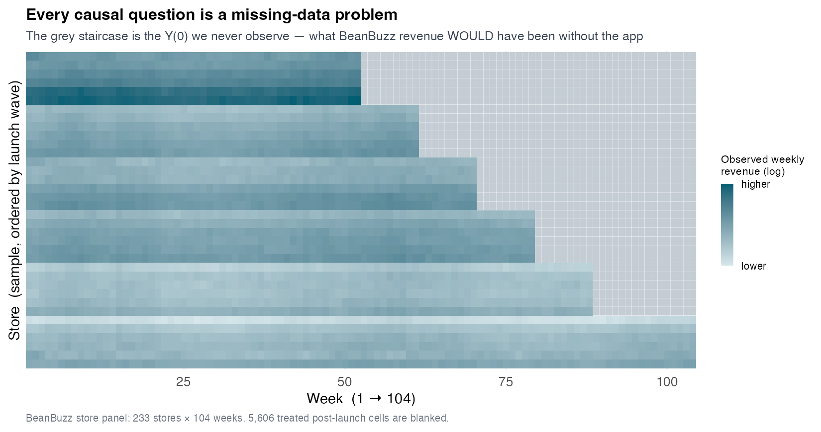
The BeanBuzz store panel: 233 stores × 104 weeks, balanced — 158 treated (staggered) + 75 never-treated.

The grey staircase is 5,606 treated cells. For each we need its untreated Y(0) — which by definition we never see.

The counterfactual is a missing-data problem

Every ATT is observed − imputed over the grey block — pick the rule that fills grey from white.

Pin the concrete object. The panel is balanced — 233 stores across all 104 weeks, no mechanical gaps; the only missingness is causal. Of the 233, 158 eventually launch the app (treated), 75 never do (the clean control pool, the white cells). Count the blank precisely: 5,606 treated store-weeks after each store’s own launch — the ragged staircase, ragged because stores launched in waves. For a treated store after launch we observe Y(1) but never Y(0), and the ATT needs exactly that. So the causal problem is literally a missing-data problem: fill 5,606 blanks. The never-treated 75 plus the pre-launch history of the treated 158 are the training set; the grey staircase is the test set. The callout is the thesis of the session in one sentence.

Settle the design, and causation becomes prediction

A refrain from week one, half-right: correlation predicts; it does not identify a cause. (Athey and Imbens 2017)

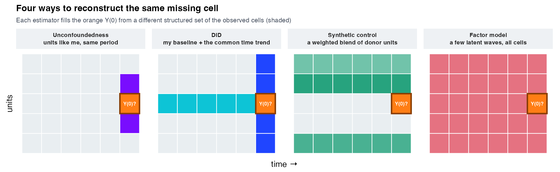
But once the design is settled — who is treated, when, which cells are clean controls — what remains is prediction: forecast the missing Y(0) from the observed cells, then subtract. (Athey et al. 2021)

Resolve the paradox students carry. All semester: “prediction is not causation” — a black-box revenue model tells you nothing about what the app DID, because it confounds treatment with everything correlated with it. That warning is correct, and it lives at the IDENTIFICATION layer: which comparisons are valid, which cells are clean controls. Once that layer is settled — and Part V settled it via parallel trends, donor hulls, factor structure — what is LEFT is a pure prediction task: use observed cells to forecast unobserved Y(0), then subtract. Both slogans true, different layers. The figure makes the shared move concrete: every panel tool since Part III predicts the SAME target cell from OTHER observed cells — unconfoundedness borrows covariate-similar units, DiD a time trend plus baseline, synthetic control a donor blend, the factor model a low-rank reconstruction. Same blank, four borrowing rules. Next: turn the four rules into one objective.

One objective fills the blank: fit the observed cells, pay for the rest

Write the untreated panel as a matrix \(L\), observed only on the white cells \(\mathcal{O}\). Every imputation estimator solves the same penalized least squares:

\[\min_{L}\ \underbrace{\sum_{(i,t)\in\mathcal{O}}\big(Y_{it}-L_{it}\big)^2}_{\text{fit the observed (white) cells}} \;+\; \lambda\cdot\underbrace{\text{penalty}(L)}_{\text{the structural assumption}}\]

\(L_{it}\) is the reconstructed \(Y_{it}(0)\): on the grey treated cells it is the imputed counterfactual, and the ATT averages observed \(-\,L_{it}\) there.

The penalty is the only thing that changes (Athey et al. 2021): the assumption on the grey cells — additivity, a fixed-rank factor, or a nuclear-norm shrink. One dial, not a menu.

This is the frame the whole session hangs on — keep it in business language. Write the untreated panel as a matrix L that we observe only on the white cells. Every imputation estimator today minimises the SAME thing: squared fit to the observed cells PLUS lambda times a penalty on the reconstruction — fit what you see, pay for the structure you assume on the cells you cannot see. The penalty IS the assumption, and it is the only moving part: strict additivity (FEct), a fixed-rank factor (IFEct), or a nuclear-norm shrink (MC). So this is not four estimators to memorise — it is ONE objective with a dial, and the next slides just turn it. Keep the scope honest: squared loss targets the MEAN Y(0), so this is specifically the outcome-model / imputation move; where it sits among the other panel families (weighting = synthetic control, S11; doubly-robust = S10; distributional = quantile effects) is the closing ledger’s job, not this slide’s — don’t spend the landscape here. The manager’s takeaway: you are always choosing an assumption about the missing cells, never just “a method.”

The penalty is a dial, not a menu

One objective, one fect() call — only the penalty argument changes (Liu, Wang, and Xu 2024):

fect(log_rev ~ app_live, data = panel, index = c("sid","week"), method = …)

Name	Idea — what it does to the latent structure	Implementation
Additive FE (FEct)	Keep no factor — strict additivity. The dial at r = 0	method = “fe”
Interactive FE (IFEct)	Keep the top-r latent factors in full, drop the rest — hard-impute; r chosen by CV	method = “ife”
Matrix Completion (MC)	Shrink all singular values by λ — soft-impute (nuclear norm); no rank to pick	method = “mc”

R and Python

Python has no fect port: the additive rung is deterministic, so pyfixest reproduces it to the digit (+4.23%); Interactive FE and MC have no packaged estimator — hand-roll numpy.linalg.svd (hard-/soft-threshold), or read the R output. (Lab 1 is bilingual; Labs 2+ are R-led.)

The unification, and the fact that it is literally one function call with a switch — the most concrete proof of “one optimization, different regularizer.”

THE CONCEPT (left). Name the three settings and what each does to the latent structure. Additive FE keeps NONE of the factors beyond the additive means — the dial at r=0. Interactive FE HARD-imputes: keep the top r factors in full, drop the rest — a best-subset step. Matrix Completion SOFT-imputes: shrink EVERY singular value toward zero by lambda — a nuclear-norm penalty. Three penalties, one dial, one estimator. This is the strongest support for the “ife/mc are extensions of the fe imputation estimator” framing: SAME objective, nested, with Additive FE the special case at the bottom.

THE MECHANICS (right). Liu-Wang-Xu’s fect exposes that one objective: hand it the same panel and toggle method. “fe” is the additive two-way-FE imputation (the +4.23% that equalled BJS and the hand-roll to the digit); “ife” adds a fixed-rank factor (rank chosen by CV); “mc” swaps the fixed rank for the nuclear norm. The choice of causal method has collapsed into one string argument.

BILINGUAL HONESTY, grounded in the labs. The ADDITIVE rung is a fixed linear operation, so Python’s pyfixest hand-rolls it and lands on the identical +4.23% — that is Lab 1, the bilingual anchor. But fect has NO Python port, so Interactive FE and MC are R-led; Python students either hand-roll the SVD with hard/soft thresholding to SEE the low-rank structure (an optional path, not a packaged estimator) or read the R output. Do not oversell a Python equivalent that does not exist.

Keep this slide CONCEPTUAL on the penalty — the singular-value pictures that make hard- vs soft-impute visible come later, and they come twice: one opens the Interactive FE section (what “low rank” means in our 233 × 104 panel), one opens Matrix Completion (what soft-impute does to every value). Do not pre-empt them here. Next we formalise each rung, starting at zero.

Additive FE

FEct forces the interaction to rank zero

Objective	\(L_{it}=\alpha_i+\lambda_t\)  (no factor)
Borrows from	my baseline + the common time trend, fit on the white cells only
Regularizes by	strict additivity (parallel trends)
Dial position	r = 0

m <- feols(log_rev ~ 1 | sid + week, data = p[app_live == 0]); p$y0_hat <- predict(m, p)

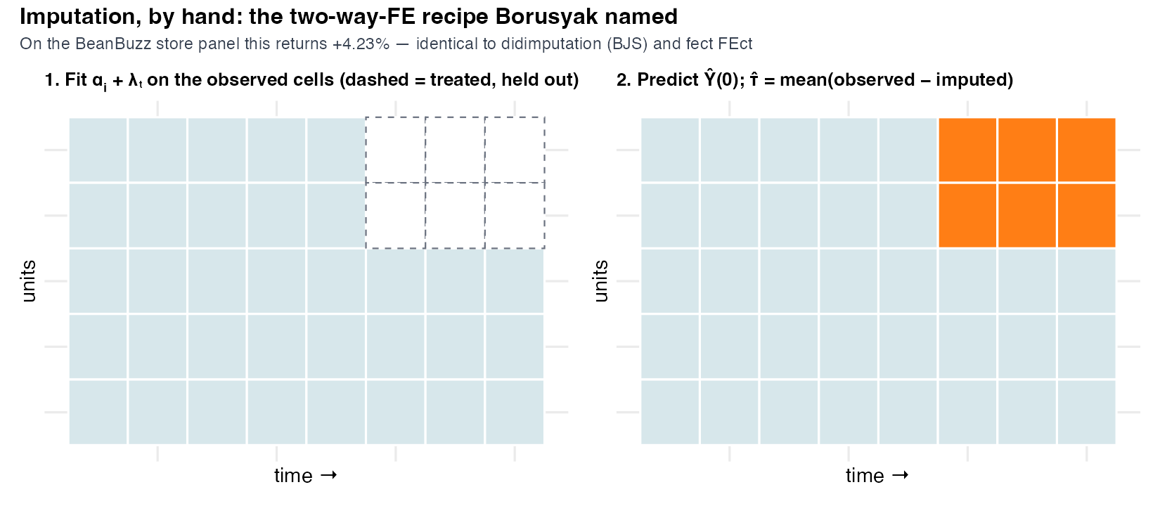
Fit on the untreated cells, predict the rest, average observed − imputed → +4.23%. This rung is the Borusyak–Jaravel–Spiess / Gardner imputation. (Borusyak, Jaravel, and Spiess 2024)

The dial at zero, formalised. The three-step recipe is exactly “fill the grey from the white”: (1) fit unit + time fixed effects on the UNTREATED cells only — the 75 never-treated stores across all weeks plus every treated store’s pre-launch history, so no treated outcome contaminates the Y(0) model; (2) predict each treated cell’s Y(0) = α̂_i + λ̂_t; (3) average observed − imputed over the 5,606 grey cells → +4.23%. The one-line code is on the slide: feols on the app_live==0 rows, then predict over the whole panel. The restriction to untreated cells is what makes the prediction a clean counterfactual rather than a tautology. Name the pedigree: this restricted two-way-FE imputation is precisely the estimator Borusyak-Jaravel-Spiess and Gardner independently proposed (the “efficient” imputation). It is a code MENTION here; the runnable bilingual version is Lab 1. Round to +4.2% in prose; keep the exact +4.23% for the identity next.

Three implementations, one number — to the digit

Three computations that look different:

• fect FEct (method="fe")
• BJS imputation (didimputation)
• hand-rolled feols + predict

all return +4.23% — max abs diff \(< 10^{-5}\).

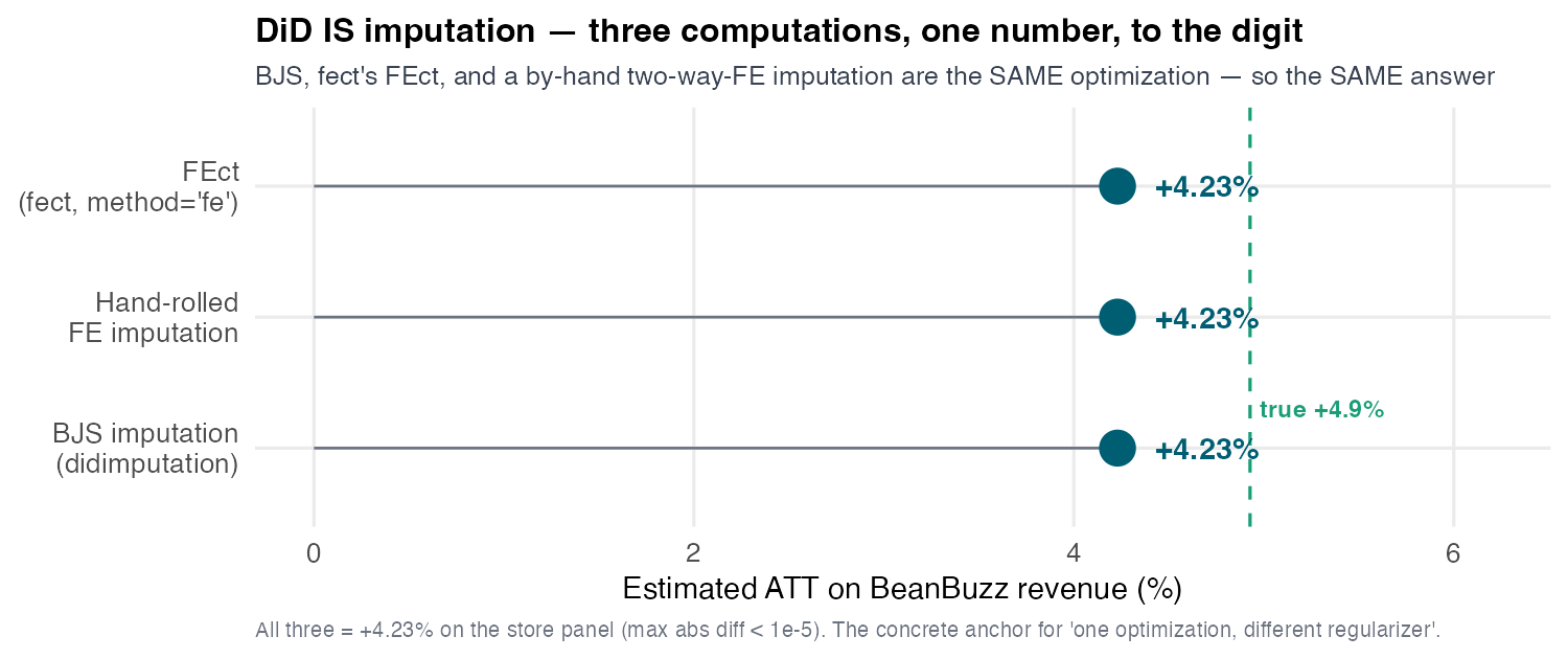
Not “about the same.” The same estimator, three ways — restricted two-way-FE imputation is a fixed linear operation, so any correct code must return it. (Gardner’s did2s lands here too — a coincidence exact only because there are no covariates.)

The anchor. Three computations that look completely different land on +4.23% with a max absolute difference below 1e-5. This is NOT three methods that agree closely — it is one estimator written three ways, and the residual is floating-point noise. Earn the phrase “to the digit”: unlike a confidence interval this identity is deterministic — restricted two-way-FE imputation is a fixed linear operation, so any correct implementation returns the same number. Be precise about Gardner: his two-stage did2s ALSO coincides here, but frame it honestly as an empirical coincidence — exact only in the just-identified, no-covariate, restricted-untreated-fit case (with covariates or a different fit sample the estimators can diverge). The payoff: DiD under two-way FE does not merely RESEMBLE an imputation — it IS one, exactly, and it is the dial at zero. Lab 1 runs the identity in R and Python. Then turn it into a question: this honest number is still too low — why?

Blind, not biased: additivity cannot see the factor

The imputation is honest — clean-cell fit, no contamination — yet it lands at +4.23%, below the true +4.93%. It isn’t biased by selection — it is blind.

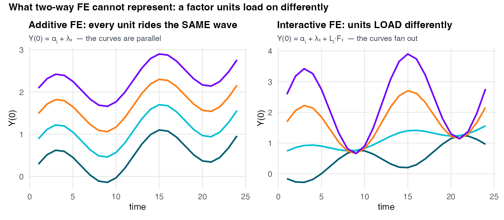
Two waves run through BeanBuzz. Whole regions boom and slump together, and some ride that cycle far harder than others — the big one. Fainter: winter footfall vs year-round routine makes urban stores ride the seasonal wave harder than roadside ones.

The loading is a β

\(Y(0)=\alpha_i+\lambda_t\) is strictly additive — every store rides the same time wiggle, so it cannot represent a latent wave \(F_t\) that stores ride by different amounts. Each store’s loading \(L_i\) is its exposure to that wave — exactly like a stock’s β on the market. Additivity forces the same β on every store, averages the factor away, and undershoots.

The cliffhanger, and it is a different villain than usual. The identity-confirmed imputation is honest in every way students have been trained to check — clean untreated fit, no selection, no forbidden comparisons — and yet it sits at +4.23%, clearly below the oracle +4.93%. This is NOT a selection artifact like the naive +16.3%. It is STRUCTURAL blindness. Two-way FE says Y(0) = unit effect PLUS time effect — strictly additive, separable — which cannot represent an interaction: a latent factor that moves over time AND that different stores load on by different amounts. Left picture: additive keeps all Y(0) paths parallel — that IS parallel trends, drawn. Right: the interactive model adds L_i·F_t and the paths fan.

THE BETA ANALOGY — lead with this, it is the fastest way to make the loading intuitive to anyone who has seen CAPM. A market-wide shock hits every stock, but each stock has its own BETA. Same here: a shared wave moves every BeanBuzz store, but each store has its own exposure to it. L_i IS a beta. Additive two-way FE is the (absurd) special case that forces beta = 1 for everyone.

WHAT THE TWO WAVES ACTUALLY ARE (verified against the DGP — say the dominant one first):

1. THE REGIONAL-ECONOMY WAVE — the BIG one, and the one the factor model will recover. A slow regional business cycle: whole regions boom and slump together, and the regions differ sharply in exposure — some ride the cycle hard, one barely moves at all. In the data this is unmistakable: the loading on this wave is explained by REGION with R-squared 0.97. Economically it is the most familiar factor there is — a regional downturn hits every store in that region at once, and how hard depends on what that regional economy is made of.

2. THE COFFEE-SEASONALITY WAVE — real, but the FAINTER one, and the reason this is subtle. Cold, dark months lift hot-drink demand everywhere. But the common time effect lambda_t ALREADY absorbs the AVERAGE seasonal lift — so seasonality only survives as an interaction to the extent that stores ride it by DIFFERENT amounts. That differential is genuine but small: a downtown, pedestrian store sells impulse cups to people literally outside in the cold (high exposure); a roadside drive-through sells the habitual commuter’s cup from a heated car (low exposure). Concretely: a high-urban store swings roughly 16% peak-to-trough, a roadside one about 11%, and in our data the seasonal swing runs ~15% (least-urban third) to ~18% (most-urban). Real — but the spread in regional exposure is roughly 6-8x larger, which is why seasonality is the SECOND factor, not the first.

THE PAYOFF OF GETTING THIS RIGHT: r = 1 will catch the regional wave and leave the seasonality behind — and that leftover is exactly what the placebo fires on later. The two waves are not decoration; they are the plot.

The fix is not better fitting but a richer model — turn the dial up.

Interactive FE

Low rank: the panel hides in two thin matrices

Both panels are one tool: the singular value decomposition (SVD). Split a matrix into \(U\Sigma V^{\top}\), keep the top \(r\), and you have the two thin matrices — \(\Lambda = U_r\Sigma_r\), \(F = V_r^{\top}\) — while the \(\sigma_k\) on the right are its spectrum. And \(\Lambda F\) is defined on every (store, week), including the 5,606 blanked cells: multiply, and the blanks are filled. That is completion.

Make “low rank” concrete before we formalise the estimator — this is the picture the whole section rests on. Two moves, one figure — and ONE tool underneath both: the SINGULAR VALUE DECOMPOSITION.

NAME THE TOOL. Both halves of this figure are SVD. Any matrix factors as U Sigma V-transpose: orthonormal columns, and a diagonal of singular values ordered largest to smallest. Keep only the top r and you have exactly our two thin matrices — Lambda = U_r Sigma_r (233 x r), F = V_r-transpose (r x 104). The bar chart on the right is literally that Sigma. And the truncation is not a heuristic: by Eckart-Young, the rank-r truncated SVD is the BEST rank-r approximation of the matrix in least squares. So “low rank” and “SVD” are the same sentence said twice.

SVD IS THE ENGINE UNDER BOTH RUNGS — this is the payoff of naming it, and it sets up the next two sections. Interactive FE HARD-thresholds the singular values (keep the top r in full, drop the rest = truncated SVD). Matrix Completion SOFT-thresholds them (subtract lambda from every one = the prox operator of the nuclear norm). Same decomposition, two ways to cut it. When we get to the MC slide, that is all “soft-impute” means.

ONE HONEST NUANCE — do not let a sharp student catch you here. You cannot take a single SVD of Y(0), because Y(0) HAS HOLES (the 5,606 treated cells). The algorithms therefore ITERATE: fill the missing cells with the current estimate, take the SVD, threshold the singular values, re-impute, repeat until it settles. That is exactly what fect does internally (EM / soft-impute). The spectrum plotted on the right sidesteps this by using the COMPLETE never-treated block (75 stores x 104 weeks, no missingness), where a single SVD is well defined — which is why the panel is labelled that way. Name the function out loud — numpy.linalg.svd / R’s svd() — because it is the engine under both rungs, but do not promise a Python lab path: fect has no port, and Lab 2 is R.

FACTORIZATION (left). Take the untreated panel Y(0): 233 stores down, 104 weeks across — say the dimensions out loud, because the shape is the whole point. Strip the additive part (alpha_i + lambda_t) — that is FEct, the dial at zero. What is LEFT is not noise: it is a matrix of essentially rank one, which means it can be written as a TALL THIN column times a WIDE FLAT row. Lambda is 233 x r — one loading per store, how hard that store rides the wave. F is r x 104 — one value per week, the wave itself. That is the entire interaction: a store-specific loading times a common time factor. A 24,232-cell matrix compressed into 233 + 104 numbers.

COMPLETION (the punchline). Here is why this buys us the counterfactual: Lambda and F are defined for EVERY store and EVERY week — including the 5,606 store-weeks we blanked. Nothing in the product needs the treated cells. So estimate Lambda and F from the cells we DO see, multiply them out, and the blanked cells are simply… filled. That is matrix completion: not a trick, just a low-rank object evaluated where we had no data.

THE SPECTRUM (right) — and these are OUR numbers, computed from the BeanBuzz panel, not a textbook cartoon. Take the never-treated block (75 stores x 104 weeks, complete, no missingness), de-mean it two ways, and take the SVD. The first singular value TOWERS: it alone carries 50% of the residual variance. Singular values two through eight sit on a flat noise floor, each around 2-3%. That gap IS the low-rank structure, and it is why cross-validation picks r = 1 — the dominant wave (the regional-economy cycle) is the only one that stands clear of the noise floor. (The DGP does hide a genuine SECOND wave — the coffee seasonality — but its differential exposure is 6-8x smaller than the regional one, so it is buried in that floor. It is too faint for CV to buy a second factor for it, and that is precisely why the placebo will fire small later.)

So: rank is not an abstraction you assume; it is something you can LOOK at. The next slides formalise the estimator that exploits it.

IFEct hard-imputes a rank-r factor — CV picks r = 1

Objective	\(L_{it}=\alpha_i+\lambda_t+\sum_{r} L_{ir}F_{rt}\)
Borrows from	a few shared latent factors everyone loads on
Regularizes by	a fixed rank \(r\) (hard-impute), CV-chosen
Dial position	r ≥ 1  (FEct is \(r=0\))

So which \(r\)? Cross-validation — no oracle needed: hide a block of pre-launch weeks you do observe, re-impute them at each candidate \(r\), and keep the simplest \(r\) whose held-out error is within one SE of the best. Here it picks r = 1. (Xu 2017; Liu, Wang, and Xu 2024)

plot(out.ife, type = "factors") — but read the legend twice.

0 is not a factor. It is the time effect \(\lambda_t\) — loading 1 for every store. A lift. The additive model already had it.

1 is the one CV bought. Its loadings run \(-0.069\) to \(+0.027\) — 18% negative. Same week, opposite directions.

A fan, not a lift — and that is what additivity cannot see.

Turn the dial to r ≥ 1, and land the “aha” in the same breath. IFEct adds the term the additive model was missing: L_i·F_t — a store-specific loading (the beta) on a shared time-varying factor. Objective, borrows-from, regularizes-by: the same card template as FEct, one row richer. The regulariser is a FIXED RANK r — keep the top r singular values in full, drop the rest (hard-impute, i.e. a truncated SVD). Emphasise the nesting: FEct is exactly this at r = 0, so IFEct is the extension, not a different animal.

CROSS-VALIDATION, in one line here — the full recipe is on the face of the NEXT slide, so do not spend the room’s patience twice. We never look at the truth; we manufacture a test set from data we already have, by hiding three consecutive PRE-LAUNCH weeks in a sample of stores, deleting everything after them from training, and scoring each candidate r on how well it FORECASTS them forward. On BeanBuzz it picks r = 1. (Next slide: the recipe, and the whole band across r.)

THE FIGURE IS fect’s OWN — plot(out.ife, type = "factors"), nothing hand-drawn. And it comes with a TRAP that you must spring yourself, out loud, before a student springs it on you. It draws TWO lines and legends them “Factor(s) 0” and “Factor(s) 1” — on a fit where CROSS-VALIDATION PICKED ONE FACTOR. So: what is line 0?

LINE 0 IS NOT A FACTOR. It is the two-way TIME FIXED EFFECT, lambda_t. I verified it against the fitted object: identical(series_0, f$xi) is TRUE, correlation 1.0000. fect indexes it as “factor 0” because, formally, a time effect IS a factor whose loading is FIXED AT 1 for every unit — but that is exactly what makes it NOT the thing we came here for. Every store gets it, in full, in the same direction. It is a LIFT. The additive model ALREADY HAD IT; FEct has lambda_t too. And note the cruelty of the picture: line 0 is the BIGGER-looking curve (sd 0.052 vs 0.031 on this scale), so the eye lands on it first and reads it as “the factor.” It is not. BELIEVE THE OBJECT, NOT THE LEGEND — the same discipline as the mistitled sensitivity plot later in the deck.

LINE 1 IS THE ONE CV BOUGHT — and the way to see that it is a different KIND of thing is to look at its LOADINGS, not at the curve. The loadings run from -0.069 to +0.027, and 18% OF STORES LOAD NEGATIVE. So in the same week, as line 1 rises, roughly one store in five goes DOWN while the rest go UP. That is a FAN, not a lift — and a fan is precisely what an additive model cannot represent, because additivity forces one common time path on everybody (the “blind, not biased” slide, three slides back: the loading IS a beta). THAT is the term IFEct adds. Say it in one sentence: line 0 is the wave everyone rides together; line 1 is the wave they ride against each other.

TWO CAUTIONS ON READING LINE 1. (a) Its sign and scale are ARBITRARY — the factorization identifies only the PRODUCT L_i*F_t, so flipping the sign of both the loading and the factor changes nothing. Never read the y-axis on its own; always read it THROUGH a loading. (b) The curve is the wave’s SHAPE; which way a given store actually moves is the loading’s job.

AND WHICH WAVE IS IT? (Podium only — the figure no longer shows this, and it should not.) It is the slow REGIONAL-ECONOMY cycle: its loading is explained by region (R-squared 0.97) and it correlates only +0.10 with the seasonality cosine — which is why the trace is a wiggly, persistent drift rather than a clean annual sine. Against the ORACLE factor it lands at correlation 0.999. Say that number if you want to make the recovery vivid, but say WHERE it comes from: it is visible only because this world is simulated. A practitioner has no such check, and the slide is now honest about that — the FACE makes its case from the loadings, which any student can compute on their own screen. Recovery of the factor is the MECHANISM; the estimate climbing (+4.23% → +4.76%) is the RESULT.

Plant the honest caveat now, because it is the SETUP for the sensitivity section: r = 1 buys you exactly ONE factor, and it spent it on the regional wave. The COFFEE-SEASONALITY wave — the weaker second factor, the one urban stores ride harder than roadside ones — is left behind. That leftover is precisely what the placebo will fire on (+0.78%, p = 0.002), and refitting at r = 2 absorbs it. The placebo is not a mystery; it has a name.

(If a student asks about gsynth: it is not a fourth method. Xu’s generalized synthetic control is this same interactive-FE model with the factors estimated from the never-treated cells only; fect subsumes it, so we teach one estimator. Kept off the slide deliberately.)

Turn the dial: CV picks the rung, not the oracle

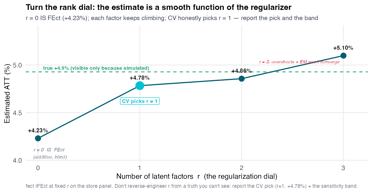
You pick the rung without the truth line:

1. Hide a 3-week block of observed, pre-launch weeks in 10% of stores — and delete everything after it from training.
2. Re-impute the block at each candidate \(r\); score the held-out error.
3. Keep the simplest \(r\) within one SE of the best — here r = 1.

Refit at fixed \(r\) and the estimate is a smooth function of the regularizer: r = 0 IS FEct (+4.23%) → r = 1 +4.78% → r = 2 +4.86% → r = 3 +5.10% (overshoots; the EM stops converging).

Report what CV gave you, not what the oracle knows

CV picks r = 1 → +4.76%. You know — only because this is simulated — that r = 2 lands nearer +4.9%. A practitioner has no truth line. Report the CV pick; never reverse-engineer the rank from an answer you cannot see.

The dial, and the tuning question answered — this is the slide the old deck buried inside “Sensitivity,” where it never belonged. Turning the rank dial is MODEL SELECTION, not a stress test of an assumption; it asks “which rung fits best,” and that is a different question from “what does the rung I picked still fail to see.”

THE NESTING PROOF, first, because it is the most convincing picture in the act. Refit IFEct at each fixed rank and plot the ATT against r. At r = 0 the estimate is EXACTLY the FEct number, +4.23% — the dial at zero literally reprints the additive imputation. The whole family is one estimator with one knob, and you can see it in one line.

Turn the knob: r = 1 gives +4.78%, r = 2 +4.86%, r = 3 +5.10% — smooth, climbing, and by r = 3 it OVERSHOOTS the truth and the EM algorithm stops converging (over-ranked, poorly conditioned). One number to be scrupulous about, because two live in the cache and they are NOT the same: the dial’s r = 1 is +4.78% — a FIXED-r refit — while the headline IFEct estimate is +4.76%, the CV-SELECTED fit. Different EM runs, same rank. Quote +4.78 on the dial, +4.76 as the answer. Do not let them merge.

CROSS-VALIDATION — say it slowly, because students meet “CV picks r” as if it were magic, and the details matter more than they look. We do NOT get to look at the truth. So we manufacture a test set out of data we already have. But note WHAT fect hides, because it is not what most people assume: it does not scatter blanks across the panel. It samples 10% of the stores, hides a CONTIGUOUS three-week block of their PRE-LAUNCH weeks, and then deletes everything AFTER that block from the training window — so the model has to FORECAST FORWARD across a gap onto cells it was denied. That geometry is deliberate: it mimics the shape of the real job (fit on the pre-period, extrapolate into the post-period) instead of filling scattered interior holes. It is honest precisely because it never touches a treated post-launch cell or the oracle — it is judged on prediction, not on the answer we want.

AND THE KEEP-RULE IS NOT THE ARGMIN. fect’s default is cv.rule = “1se”: it keeps the SIMPLEST model whose held-out error is within one standard error of the best, not the outright winner. On BeanBuzz that is r = 1 — a second factor does not improve held-out prediction enough to earn its place, because the second wave is weak. (On the MC ladder two slides from now you will WATCH this rule reject the lowest-scoring lambda. Do not say “keep the r that predicts best” — the deck will contradict you on screen.)

THE DISCIPLINE, and this is the exact skill A5 grades: you report what CV gave you (+4.76% at r = 1), NOT the oracle-informed r = 2 (~+4.9%) — because a practitioner has no truth line to reverse-engineer the factor count from. The oracle line on this figure is dashed and labelled “visible only because simulated”; in A5 there is none. The small residual gap between the r = 1 estimate and the truth is not a bug to fix by peeking. It is the honest cost of not knowing how many factors the world has.

Hand over deliberately, because the next act asks a genuinely different question: the dial answers WHICH RUNG FITS BEST. It says nothing about what the rung you picked still cannot see — or what that blindness costs. That is the sensitivity act, and it opens by dissolving an objection you should already be feeling.

+4.76% is the average of a ramp — not a level

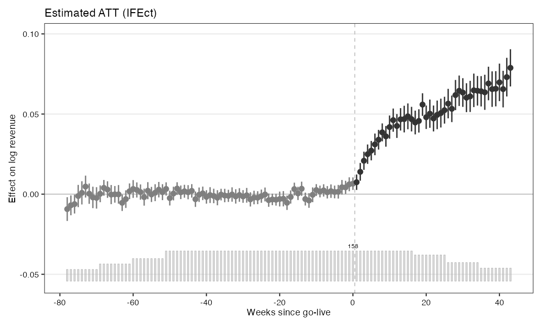
plot(out.ife, main = "Estimated ATT (IFEct)")

Before: flat on zero. That flatness is a claim — the Sensitivity act audits it.

After: a ramp, not a jump — +0.7% wk 1 → +4.3% wk 12 → +6.6% wk 52.

Adoption is a diffusion, not a switch.

So +4.76% is not “the effect.” It is the mean over the post-window you chose — and the window is a choice.

The fit, drawn by fect itself — one call, no hand-rolling. And it does something a single number cannot: it puts the estimate’s SHAPE on screen. Spend a moment here, because two of the deck’s remaining three acts are set up on this picture.

READ THE LEFT HALF FIRST — the pre-launch weeks. They sit flat on zero, with tight intervals. Students will read that as reassurance: “no pre-trend, we’re fine.” Do NOT let that land as a verdict. It is a CLAIM, and the entire Sensitivity act exists to interrogate it — the placebo will blank three of those weeks and re-impute them, and it will FIRE (p = 0.002). Flat to the eye is not flat to a test. Plant that now; you will collect on it in two acts.

READ THE RIGHT HALF SECOND — and notice it is a RAMP, not a jump. Week 1 is +0.7%. Week 12 is +4.3%. By week 52 it is +6.6% and still climbing. That is what app adoption actually looks like: customers download, habituate, re-order — a diffusion, not a switch that flips. Almost nothing in a business rolls out as a step function, and an event-study plot is the cheapest way to see it.

NOW THE PUNCHLINE, and it is the one to say slowly: +4.76% IS AN AVERAGE OVER THIS RAMP. It is not “the effect of the app.” Average over weeks 1-12 and you get one number; average over the full 52 and you get a bigger one; average over week 1 alone and you get +0.7%. The estimand is not handed to you by the estimator — YOU PICK IT, when you pick the window. This is the exact point the Heterogeneity act closes on (“the penalty was the assumption; the restriction was the assumption; the AGGREGATION is the question”), and it is worth planting the seed here rather than springing it at the end.

(One honest note on the x-axis, if a sharp student asks: the window runs out to event week -87, but those far-left cells are THIN — only a handful of stores are observed that long before their own go-live, which is what the grey histogram along the bottom is telling you. The count peaks at 158 stores around go-live. That thinning is not cosmetic: in the Sensitivity act, ONE argument — proportion 0.3 -> 0.5 — drops the thinnest of those weeks and flips the pre-trend verdict. The picture you are looking at already contains that fragility.)

Matrix Completion

MC soft-imputes by shrinking the singular values

The nuclear norm = the sum of a matrix’s singular values; penalizing it shrinks them toward zero. That is what “encourages low rank” — and it is the same objective, a softer knob. (Athey et al. 2021)

Objective	\(\min_L \sum_{\mathcal{O}}(Y-L)^2 + \lambda\lVert L\rVert_{*}\)
Borrows from	a low-rank reconstruction — all factors, shrunk
Regularizes by	the nuclear norm \(\lVert L\rVert_*\) (soft-impute), CV-\(\lambda\)
Dial position	soft — and MC → FEct once \(\lambda\) exceeds \(\sigma_{\max}\)

Nested, to the boundary

Push \(\lambda\) past the largest singular value and every factor is shrunk to zero — MC collapses back to FEct. Hard-impute keeps a few factors whole; soft-impute keeps all of them, smaller.

The third rung, and the last piece of the nesting. Matrix completion swaps the fixed rank for a nuclear-norm penalty — the sum of singular values — and minimises fit-plus-penalty. Where IFEct hard-imputes (keep the top r values in full, drop the rest), MC soft-imputes (shrink ALL values by lambda). Same objective, softer knob. Close the nesting explicitly: as lambda grows past the largest singular value, every factor is shrunk to zero and MC reduces exactly to FEct — the whole ladder collapses to the dial at zero. This is Liu-Wang-Xu verbatim and it is why “one estimator, one dial” is literally true, not a metaphor.

THE FIGURE (upper right) — make the penalty VISIBLE on the same singular-value picture we have been building. Interactive FE hard-imputes: keep the top r singular values IN FULL, throw the rest away — a best-subset step (the cyan dashed path). Matrix completion never chooses a rank at all: the solution to the nuclear-norm problem is SOFT-THRESHOLDING — subtract the same lambda from EVERY singular value and floor at zero. That is what the orange arrows show: identical drops off every bar. No rank switch anywhere; the shrinkage does the work.

WHY THAT IS SEDUCTIVE. It sounds strictly better — no arbitrary rank to pick, everything tuned continuously by lambda, and the noise floor gets crushed automatically. And the noise floor DOES get crushed: look at values two through eight.

WHY IT BACKFIRES HERE — the honest counterweight, and the point to land aloud since it is no longer written on the slide. Lambda does not know which singular value is signal and which is noise. It comes off sigma-one TOO. Our sigma-one IS the regional-economy factor — the dominant thing additivity was blind to, the thing we came here to recover — and soft-impute hands back a DAMPED version of it. So matrix completion, the most flexible tool on the ladder, lands at +4.31%: barely above FEct’s additive +4.23%, and well short of IFEct’s +4.76% against a true +4.93%. The penalty that buys the flexibility also dampened the signal. Say the three numbers off the figure’s subtitle; do not let students leave thinking MC recovered the truth. It did not.

The five-word lesson, which the next slide hammers: MORE FLEXIBLE IS NOT MORE RIGHT. Flexibility must be TUNED, not assumed — a bigger hypothesis space can under-fit if its regulariser pulls the wrong way.

(Honesty note on the figure: lambda is drawn at an illustrative level — fect’s CV-chosen lambda lives on its own internal scale — but the singular values themselves are OUR panel’s, and the three ATTs are the real cached numbers.)

Same panel. Same picture. A different number.

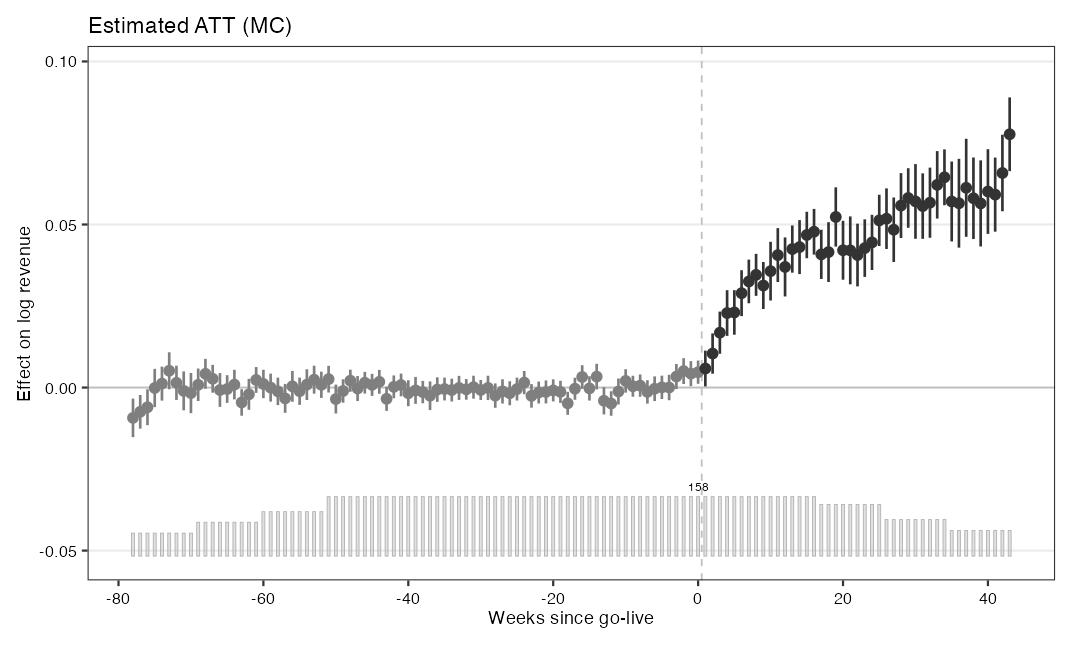
plot(out.mc, main = "Estimated ATT (MC)")

Flat before. Ramps after. The same shape — the two post-launch paths correlate 0.99.

ATT	95% CI
IFEct +4.76%	[+4.23, +5.28]
MC +4.31%	[+3.73, +4.89]

The eye cannot choose. Neither can the interval.

Each CI contains the other’s estimate. The whole disagreement — 0.45 pp — is smaller than a single CI half-width (0.53 pp). Two models, one panel, one picture, two answers — and nothing you can see separates them.

The same call, the same panel, the same estimand — and one string changed. Put this slide directly beside the last one in the room’s memory, because the whole point is that you CANNOT TELL THEM APART.

FIRST, the shape. Flat before, ramping after. Visually it is the previous slide. That is not sloppiness on my part and it is not a coincidence: I measured it — the two post-launch event-study paths correlate 0.99 (0.988 over the post weeks, 0.998 over the full window). Both models fit the observed cells well. THAT IS WHAT FITTING DOES. The observed cells are where they agree, by construction.

SECOND, the numbers — and this is where the slide bites. IFEct says +4.76%, 95% CI [+4.23, +5.28]. MC says +4.31%, 95% CI [+3.73, +4.89]. Look at what those intervals DO: MC’s interval comfortably contains IFEct’s point estimate, and IFEct’s comfortably contains MC’s. They overlap across almost their whole length. The entire quarrel between the two estimators — 0.45 percentage points — is SMALLER THAN A SINGLE CONFIDENCE-INTERVAL HALF-WIDTH: IFEct’s half-width alone is 0.53 pp. The disagreement between the two models is smaller than the noise in either one of them. If you handed a board these two event studies with the titles removed, no one in the room could tell you which is which, or which to trust.

SO STATE THE PROBLEM CLEANLY, because it is the hinge of the whole act: two models, one panel, one picture, two answers — and NOTHING YOU CAN SEE SEPARATES THEM. Not the fit to the observed cells (identical). Not the event-study shape (correlation 0.99). Not the confidence intervals (overlapping). The 0.45 pp lives ENTIRELY on the grey cells — the imputed Y(0) for treated store-weeks — which is exactly where no picture can go, because there is nothing there to plot.

RESIST THE TWO CHEAP ANSWERS. (a) “The CIs overlap, so the difference isn’t significant, so it doesn’t matter.” Wrong twice over: overlapping intervals are not a test of equality, and more importantly the difference is not about significance — it is about which imputation is RIGHT, and the CI is silent on that. (b) “Take the more flexible model.” Hold that thought for exactly two slides.

AND HAND OVER. If neither the picture nor the interval can choose, what can? The next slide answers it: cross-validation, which is the one thing here that scores the models on data they were DENIED rather than on data they were fitted to. It will rank them — honestly, with no oracle. And then it will refuse to certify the winner. Set that up as a genuine question, not a rhetorical one: the room should WANT the next slide.

CV also picks the family — no truth line needed

One call — fect(method = "both") — builds the folds once, then races both ladders over them.

IFEct — turn \(r\)

\(r\)	held-out MSPE
0	0.00171	= FEct
1	0.00105	kept
2	0.00116
3	0.00118
4 · 5	0.00154 · 0.00199

MC — turn \(\lambda\)

\(\lambda/\sigma_{\max}\)	held-out MSPE
1.00	0.00171	= FEct
0.42	0.00149	kept
0.18	0.00137	lowest
0.075	0.00149
0.032 · 0.013	0.00160 · 0.00166

Both ladders open on the same rung and the same score — \(r=0\) is \(\lambda=\sigma_{\max}\) is FEct, 0.00171 on each. That identity is the proof they share one ruler. And MC keeps 0.42, not its lowest 0.18: fect’s rule is one-SE, not argmin.

fect’s own verdict: “Recommended method through cross-validation: ife” → r = 1, +4.76% — the headline, chosen with no oracle.

CV can RANK — nothing can ACQUIT

The race is run on 345 pre-launch weeks — not one treated post-launch cell is ever scored. Held-out fit ranks the candidates. It never certifies the winner.

The professor’s question, answered on one slide: CAN you choose between IFEct and MC without ground truth? Yes — and fect will do it for you, in one argument. But be precise about what the answer is worth, because this slide is the setup for the next one.

ONE CALL, ONE SET OF FOLDS. method = “both” is not a fourth estimator; it is a race. fect builds the held-out folds ONCE — before it branches to either family — then runs the whole r-ladder and the whole lambda-ladder over those same hidden cells, and reports which family scored better. That shared-fold design is the ONLY reason the two columns can be compared at all.

SAY THIS OUT LOUD, because the naive version of this slide is WRONG and the error is invisible. If you call fect twice — once with method=“ife”, once with method=“mc” — the two calls draw their folds from the ambient RNG stream one after the other (fect’s seed= argument seeds the BOOTSTRAP, not the cross-validation), so they hold out DIFFERENT cells. On this panel I measured it: the two fold sets share THREE cells out of about 345. They are essentially disjoint. And here is what that costs: the SAME model — FEct — scores 0.00171 on one fold set and 0.00187 on the other. A 9% gap, out of nothing but which cells got hidden — and that is the SAME size as the real gap between the two families. Two separately-fitted MSPEs put side by side would be a race on two different racetracks, and the noise would be as big as the signal. Use method = “both”, or reset set.seed() immediately before each call.

THE IDENTITY IS THE PROOF — and it is the best thing on the slide. Both ladders NEST FEct. IFEct at r = 0 is FEct (the dial at zero, from two slides ago). And MC at lambda = sigma_max is FEct too — that is exactly the “nested, to the boundary” callout on the previous slide: push lambda past the largest singular value and every factor is shrunk to zero. Same model, two entrances. So if — and only if — the two ladders were scored on the same hidden cells, those two rows MUST report the same number. They do: 0.001713945337004485, both, to the last bit. identical() returns TRUE. That equality is not a coincidence to be admired; it is the receipt that the comparison is legitimate. If a student ever compares two CV numbers, this is the check to make them run.

THE ONE-SE RULE — the correction, and the reason “lowest MSPE wins” is not what the package does. fect’s default is cv.rule = “1se”: it does not keep the argmin, it keeps the SIMPLEST model whose held-out error is within one standard error of the best. Watch it fire on the MC ladder, live: MC’s lowest MSPE is at lambda/sigma_max = 0.18 (0.00137) — and fect REJECTS it, keeping 0.42 (0.00149), a strictly WORSE score, and printing “[cv.rule = 1se] lambda.cv adjusted (1-SE band)”. Why would anyone do that? Because a difference of 0.00012 with a standard error of 0.00019 is not a difference; chasing it is chasing noise, and the more-shrunken model is the more defensible one when the data cannot tell them apart. That is a lesson about model selection generally, and it is why the deck no longer says “keep the r that predicts best” — it says “keep the simplest r within one SE of the best.”

THE VERDICT, AND ITS PRICE. IFEct’s best (0.00105) beats MC’s best (0.00137) by about 24%, and the gap is 3.1x IFEct’s own fold-SE, so on these folds it is not noise. fect prints its recommendation without being asked. And the number it hands back — r = 1, +4.76% — is the deck’s headline, reached with no truth line anywhere in the calculation. That is the honest, field-runnable answer to “which model?” and it is what A5 rewards.

HOW ROBUST IS THE VERDICT? Be honest and be specific. I re-ran the race on 30 different fold draws: CV picks IFEct on 29 of them (97%, 95% CI 83-100%). On one draw (seed 1) MC wins and fect hands back +4.31% instead. So the ranking is strong but not deterministic — it is a property of the folds you happened to draw, and a practitioner who reran this with a different seed could, once in a while, ship a different headline. Say “CV prefers IFEct here, on almost every fold draw” — never “CV settles it.”

NOW THE REFUSAL, and hand it straight to the next slide. Every one of those 345 held-out cells is an OBSERVED, PRE-LAUNCH week — 23 stores per fold, a contiguous three-week block each, with everything after the block deleted from training so the model has to forecast FORWARD. That design is deliberate and it is the best defence of the whole exercise: it mimics the shape of the real job (fit on the pre-period, extrapolate into the post-period) rather than filling scattered interior holes. But it CANNOT close the gap that matters. The estimand needs Y(0) on TREATED, POST-LAUNCH cells — for stores that SELECTED INTO treatment, at event times with no observed counterpart. CV never scores a single one of those, and it never can: they are exactly the cells that do not exist. So a model can win this race and still impute the counterfactual worse. Held-out fit RANKS. It does not CERTIFY. The next slide shows what that costs: the most flexible tool on the ladder, MC, is the one that under-recovers — and no amount of held-out fit was ever going to tell you that in advance. More flexible isn’t more right.

Seeing the factor closes the gap — but more flexible isn’t more right

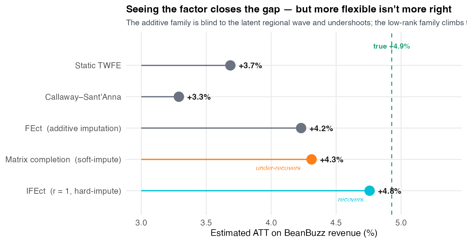
Additive family (blind to the latent wave) undershoots; IFEct +4.76% recovers; but matrix completion +4.31% under-recovers — its nuclear norm shrank the very factor we needed. More flexible ≠ more right.

The payoff of the low-rank act, delivered as two clusters — not a monotone climb. The additive family is blind to the latent regional wave and undershoots: static TWFE +3.7%, Callaway-Sant’Anna +3.3% (note it sits BELOW TWFE — additive estimators are not monotone among themselves), and the FEct imputation +4.23%. The low-rank family sees the factor: IFEct climbs to +4.76%, recovering most of the gap to the true +4.93% — IFEct is the hero here, the estimator that recovered the factor and the truth together. Now the discipline lesson, non-negotiable: matrix completion, the MOST flexible tool on the slide, lands at +4.31% — barely above the additive number, UNDER-recovering. Why? Its nuclear-norm penalty shrinks the singular values toward zero, and in doing so it shrank the very factor we needed — the penalty that buys flexibility also dampened the signal. The five-word takeaway: more flexible is not more right. Flexibility must be TUNED, not assumed; a bigger hypothesis space can under-fit if its regulariser pulls the wrong way. And keep the naive +16.3% off the ladder entirely — it is selection, not an estimator to rank. Do NOT let students leave thinking MC recovered the truth. It did not.

Sensitivity Analysis

Test 1 · Placebo — it fires, and it is small

Why. The pre-period fit is in-sample — the model was fitted on those cells. So blank three you do observe and make it re-impute them out of sample.

\(H_0\) · t-test: \(\text{ATT} = 0\) on the blanked window \(\{-2,-1,0\}\).

\(H_0\) · TOST (two one-sided tests): \(|\text{ATT}| \ge \theta = 1.44\) pp.

out.p <- fect(..., method = "ife", r = 1,
              placeboTest    = TRUE,
              placebo.period = c(-2, 0))

plot(out.p, stats = c("placebo.p", "equiv.p"))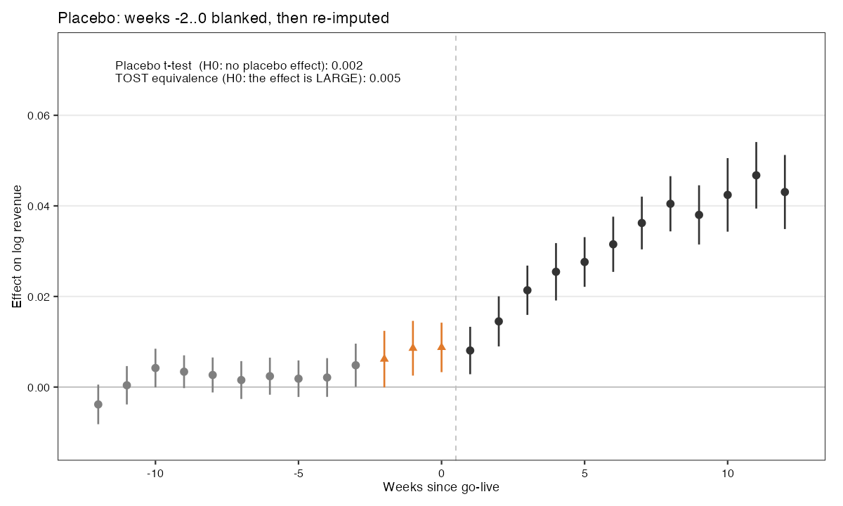

Both are true. Significance is not size.

t-test \(p = 0.002\) → reject “no placebo effect”: the violation is REAL.  ·  TOST \(p = 0.005\) → reject “the effect is LARGE”: the violation is SMALL.
A ruler, not a verdict: path \(+0.62 \to +0.86 \to +0.88\) pp ⇒ week-to-week steps \(0.240\), \(0.018\); the worst, 0.240 pp/week, denominates Test 3.

Test 1 of 4. Motivation first, and it is the same idea that runs the whole act: an in-sample fit cannot audit itself. The pre-period residuals are small partly BECAUSE the model was fitted on them. So we take three pre-launch weeks the model would normally learn from — weeks minus two through zero — declare them “treated”, and force the model to impute them from cells it was DENIED. Out of sample. That is the placebo.

READ THE TWO NUMBERS, and do not let the room collapse them into one. The t-test fires: p = 0.002. We reject “no placebo effect.” Something is there — the model mis-imputes cells it did not see. The TOST also fires, in the other direction: p = 0.005 rejects “the effect is LARGE.” So the violation is real AND it is small. Both statements are true at once, and a student who only learned “p < 0.05 = bad” cannot hold them both. SIGNIFICANCE IS NOT SIZE. Say it, write it, and come back to it.

AND NOW THE THING THAT MAKES THIS TEST DIFFERENT FROM THE OTHER THREE: it does not hand you a verdict. It hands you a RULER. The largest consecutive step in that blanked window is 0.240 percentage points per week — that is how far this model’s imputation drifts, per week, in a window where the true effect is zero by construction of the test. Hold onto that number. Test 3 does not use an absolute bound; it bounds the post-treatment violation in MULTIPLES of exactly this ruler. Every M-bar you will see in four minutes is denominated in 0.240 pp.

(Why weeks -2..0 and not some other window? It is the fect default in the docs and it is the window immediately adjacent to treatment — the hardest one to impute, and therefore the most honest ruler. Widen it and the ruler changes; say so if asked, because that is a researcher degree of freedom like any other.)

Test 2 · LOO pre-trend — nothing certifies

Why. Every pre-period so far was in-sample — the model was fitted on it. LOO re-imputes every pre-period \(t\) from a model that never saw \(t\): 88 refits, 79 tested.

out.loo <- fect(..., method = "ife", r = 1,
                loo = TRUE)

plot(out.loo, type = "equiv", loo = TRUE)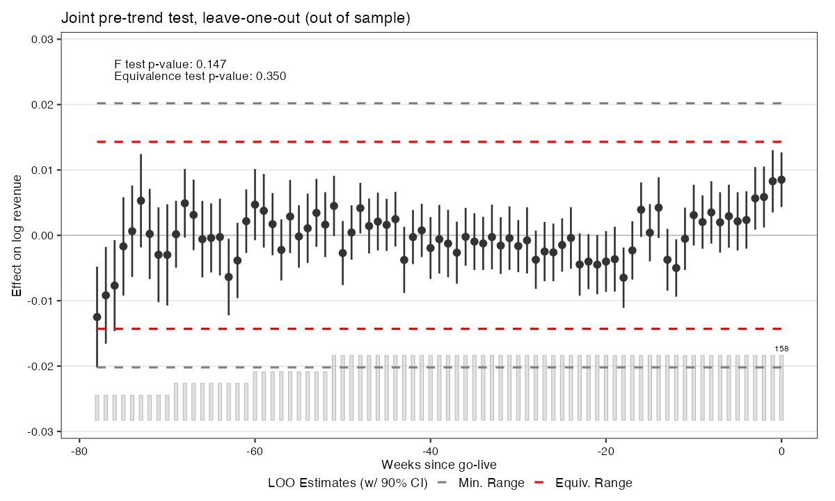

test	\(H_0\)	in-sample	LOO	what the number means
F	no pre-trend	0.126	0.147	cannot reject → absence of evidence. Never certifies.
F-equiv.	the pre-trend is LARGE	0.019	0.015	rejects → it certifies — but it averages, and averages forgive.
TOST	SOME pre-period is LARGE	0.082	0.350	cannot reject → no certificate. Intersection–union ⇒ the worst of 79, so it alone quadruples.

TOST certifies only if the grey band fits inside the red one. It does not.

Red — the bar: Equiv. Range 1.43 pp \(=0.36\,\sigma_{\text{FEct}}\) — what counts as negligible. (This fit’s own bar. Test 1’s was 1.44 — a placebo fit has a different baseline MSE, so it cuts a different bar.)  ·  Grey — the worst of the 79: Min. Range 2.02 pp \(=\max_t\big(|\hat\delta_t| + 1.645\,\text{SE}_t\big)\) — the largest violation you cannot rule out in the weakest pre-period.  ⇒  Grey sits outside red: no certificate. The two bands are the TOST — they are the 0.350, drawn.

Test 2 of 4, and it is the one that should make the room uncomfortable — because it audits the reassurance they have been leaning on since Act 1.

THE MOTIVATION, sharply: every pre-period estimate you have seen so far is IN-SAMPLE. The model was fitted on those cells. Of course the residuals are small there — that is what fitting DOES. A flat pre-trend, computed in-sample, is not evidence of parallel trends; it is partly a receipt for having run a regression. LOO removes the circularity: for every pre-period t, refit without t, then impute t. Eighty-eight refits. Genuinely out-of-sample pre-period estimates.

NOW READ THE TABLE ACROSS, and note which numbers move and which do not. The F test goes 0.126 to 0.147 — barely moves. F-equivalence goes 0.019 to 0.015 — barely moves, still certifies. And TOST goes 0.082 to 0.350 — it QUADRUPLES. Why do two tests shrug and one collapse? Because the F tests are AVERAGES over the pre-periods, and averages are forgiving: a few bad weeks get diluted by eighty good ones. TOST is an INTERSECTION-UNION test — every single pre-period must individually clear the equivalence bound, so TOST reports the WORST WEEK. In-sample the worst week was borderline. Out of sample it is not close.

POINT AT THE PICTURE AND NAME THE TWO BANDS — the room has never been told what they are, and the callout is there so you can say it in one pass.

The RED band is the BAR: 0.36 times this fit’s own two-way-FE residual SD = 1.43 pp. It is what fect is willing to call negligible, and nobody in the room chose it. ⚠️ IT IS NOT THE SAME NUMBER AS TEST 1’S — Test 1 ran on the PLACEBO fit, which blanks three weeks and therefore has a different baseline MSE, so it cut a bar of 1.44. A 0.005 pp gap you would never see, and it is the lesson: EVERY FIT CUTS ITS OWN BAR. A threshold is a property of an OBJECT, not of a session. Do not raise it unless asked, but never say “the same theta.”

The GREY band is THE WORST OF THE 79. Formally: the largest, over every tested pre-period, of |delta-hat| + 1.645 x SE — that is, the outer edge of the worst pre-period’s 90% confidence interval. Why 90 and not 95? Because a TOST at the 5% level IS two one-sided tests at 5% each, so the band is drawn at exactly the confidence level the test operates at. Read it as: THE LARGEST VIOLATION I CANNOT RULE OUT, in the weakest week I tested. Here, 2.02 pp.

NOW THE PUNCH, and it is the whole slide: TOST certifies IF AND ONLY IF the grey fits inside the red. 2.02 > 1.43, so it does not. THE TWO BANDS ARE NOT DECORATION NEXT TO THE P-VALUE — THEY ARE THE P-VALUE, DRAWN. When you say “grey inside red,” you have said “TOST certifies.” That equivalence is worth ten seconds; it is what makes the figure readable for the rest of their careers.

ONE SUBTLETY, IF A SHARP STUDENT PUSHES — and have the numbers ready, because the objection is a good one. The Min. Range mixes SIGNAL and NOISE: it is |estimate| + 1.645 x SE. So a merely NOISY pre-period inflates it even if its point estimate is dead zero. The dodge writes itself: “that is just low power in a thin cell.” IT DOES NOT WORK HERE. The worst week is event week -78, a thin cell holding 61 of the 158 stores — but decompose its 2.02 pp: the POINT ESTIMATE is -1.25 pp and 1.645 x SE is 0.77 pp. The estimate supplies 62% of the band; the standard error only 38%. It is a REAL BUMP in a thin cell, not a wide interval around nothing. Say the split out loud if challenged.

WHAT NOT TO SAY FROM THE PODIUM. It is tempting to add “and in-sample the grey band was already outside the red, at 1.52 pp, so LOO only WIDENED a failure that was already there.” That is TRUE, it is the honest reading, and it is written up in the session notes — but THIS DECK NEVER SHOWS THE IN-SAMPLE EQUIVALENCE FIGURE, so do not assert 1.52 as though the room had seen it. You do not need it. The in-sample TOST p = 0.082 IS in the table on this slide, and it carries the same point: “it did not certify in-sample either — and out of sample it is not close.” Stay on what is on the screen.

WHAT TO CONCLUDE — and be precise, because this is exactly the fallacy the course polices. Do NOT say “the pre-trend failed.” Say: NOTHING HERE CERTIFIES THE PRE-TREND. The F-equivalence still certifies out of sample (0.015) — because it AVERAGES over the pre-periods, and averages are forgiving. The TOST does not, and cannot, because it must clear the bar in EVERY ONE of the 79 tested pre-periods and reports the worst. The honest report is: the model’s out-of-sample pre-period behaviour is materially worse than its in-sample behaviour, and the in-sample number was hiding exactly that.

THE DEFECT — say it out loud, because THE PACKAGE MAKES EXACTLY THE MISTAKE THIS SLIDE IS ABOUT. Ask the plot for its numbers with return.test = TRUE and you get the CACHED IN-SAMPLE test.out: F 0.126, TOST 0.082 — the numbers the figure did NOT print. It hands you the IN-SAMPLE statistics when you asked for the OUT-OF-SAMPLE ones. That is the slide’s own thesis, committed by fect. The out-of-sample statistics live in a different slot, floo$loo.test.out. If you quote a number a package PRINTS ON A FIGURE, get it from where the figure got it. We have now been bitten by this twice (the equivalence plot’s cached test.out, and this). It is off the slide face on purpose — it changes NO number you can see, so it belongs at the keyboard: it is in the session notes and it is what Lab 3 protects you from.

Hand over: two tests have now measured the violation. Neither told you what it COSTS. That is the next two slides — and they answer it in two different currencies, and they disagree.

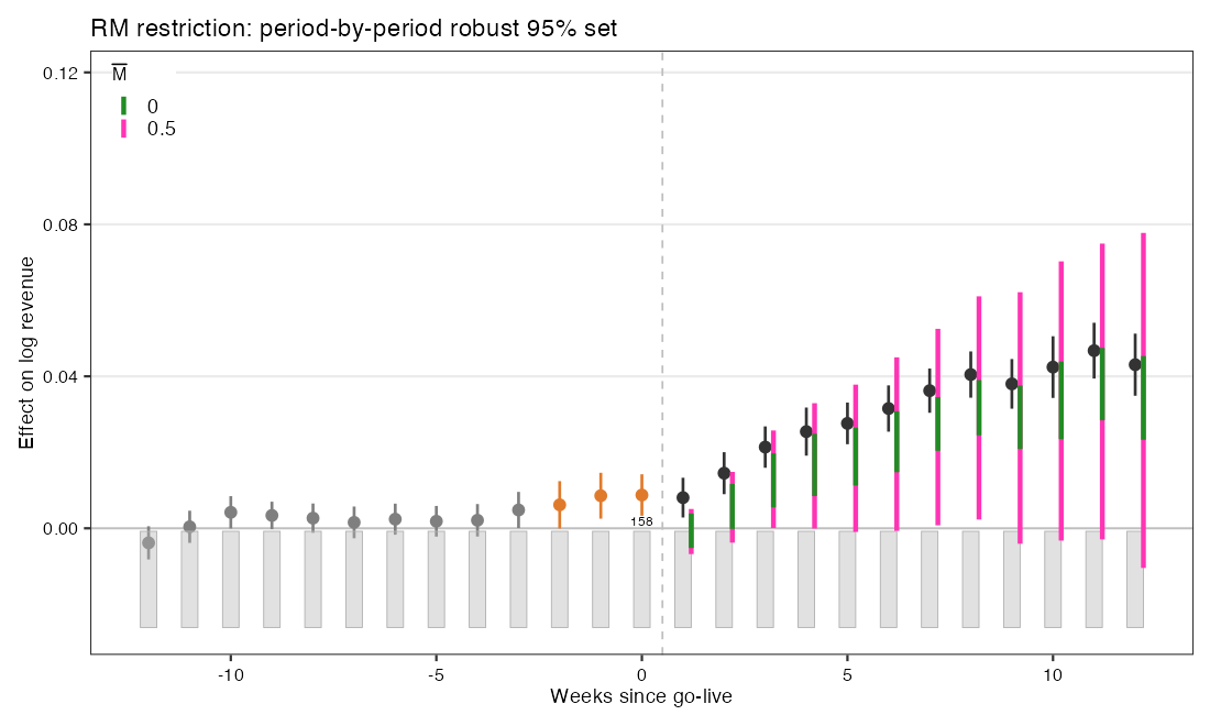
Test 3 · RM — the answer survives to \(\bar M^{*} = 0.46\)

Why. Don’t assume parallel trends — bound the violation by the drift the placebo measured: \(\Delta^{RM}(\bar M)=\big\{\delta: |\delta_{t+1}-\delta_t| \le \bar M R\big\}\), with \(R\) = Test 1’s ruler = 0.240 pp.

s <- fect_sens(out.p,
        post.periods  = 1:12,
        Mbarvec       = seq(0, 1, 0.05),
        periodMbarvec = c(0, 0.5))

plot(s, type = "sens",    restrict = "rm")
plot(s, type = "sens_es", restrict = "rm")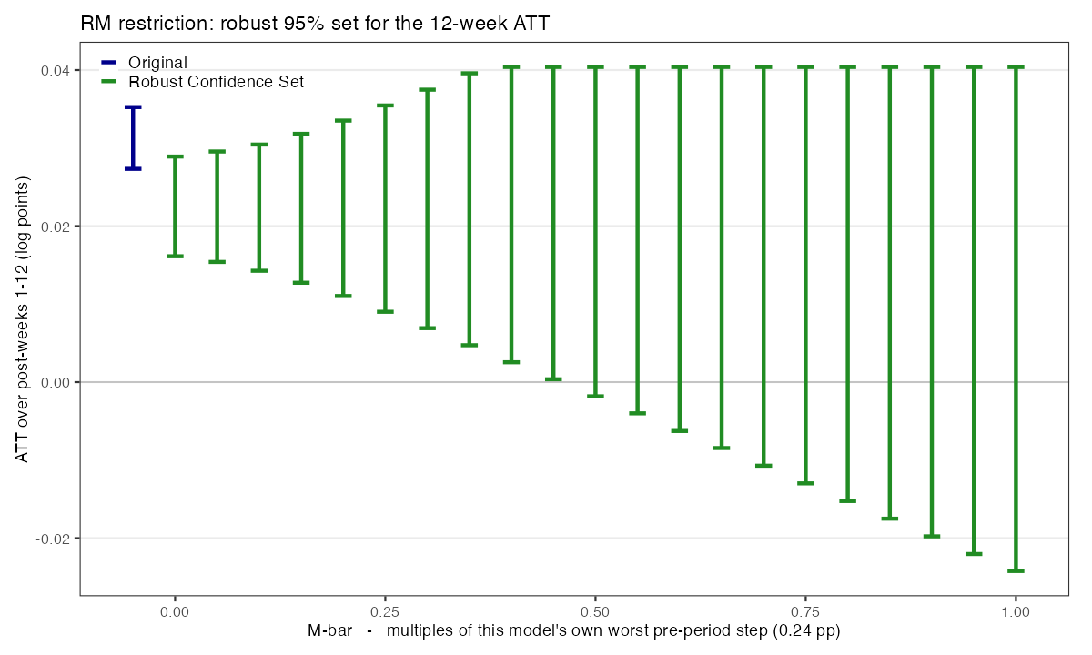

The strictest setting is not the null — and a breakdown value is only half an answer

① The freeze. Original +3.13% → at \(\bar M{=}0\): +2.25%. And \(3.13-\mathbf{0.88}=2.25\) — it subtracted \(\delta_0\). A null cannot move an estimate ⇒ \(\bar M{=}0\) freezes the violation; it does not zero it.
② The pair. \(\bar M^{*}{=}\mathbf{0.46}\) — of what? \(\bar M\) is a multiple of \(R\): \(0.46\times0.240\) pp \(=\) 0.11 pp/week. Never quote one without the other.
③ Per week (right). 2 of 12 weeks contain zero at \(\bar M{=}0\); 9 of 12 at \(\bar M{=}0.5\). A step allowance accumulates ⇒ the sets widen with the horizon.

Test 3 of 4. The first two tests MEASURED the violation. This one prices it: how big would the post-treatment violation have to be before my answer dies?

THE IDEA, in one sentence: instead of assuming delta equals zero, ASSUME LESS. Assume only that the post-launch violation does not step around more wildly than the pre-launch violation already did — by more than a factor M-bar. That is Rambachan-Roth’s relative-magnitudes restriction, and fect_sens implements it on top of the placebo fit. The ruler in the denominator is the 0.240 pp step from Test 1. That is why Test 1 had to come first.

READ THE LEFT FIGURE. As M-bar grows, the robust confidence set widens. The lower bound falls, crosses zero around M-bar 0.46, and that is the BREAKDOWN VALUE: the tolerance at which you can no longer rule out “no effect.”

NOW THREE FACTS, and they are the slide.

ONE — THE FREEZE, and this is the one that surprises everyone including me. M-bar = 0 is the STRICTEST setting. Intuitively it should reprint the original estimate. It does not: the original band centres +3.13%, the M-bar = 0 band centres +2.25%. The gap is 0.88 percentage points — and 0.88 is EXACTLY delta-zero, the last violation the placebo measured. A null assumption cannot move a point estimate. So M-bar = 0 is not “no violation”; it is “the violation stays FROZEN at whatever it was at the moment of treatment, forever.” It carries the placebo’s last step forward through all twelve weeks and subtracts it. That is a strong assumption wearing the costume of a null.

TWO — M-BAR STAR IS 0.46 OF WHAT? A breakdown value is a MULTIPLE, and multiples are meaningless without their unit. 0.46 times the 0.240 pp ruler is 0.11 percentage points per week. THAT is the answer: my estimate dies if the true post-launch trend drifts by more than about a tenth of a point per week. Report the PAIR — the multiple and the pp/week it stands for. A model that fits its own pre-window better cuts a SHORTER ruler, and therefore earns a BIGGER M-bar-star for free. Breakdown values are not comparable across models. This is exactly what A5 grades.

THREE — THE FAKE LID, and this is a package defect you can see with your eyes. Look at the top of the left figure: from M-bar 0.40 rightward, the upper bound STOPS MOVING. Thirteen of the twenty-one upper bounds are pinned to the same number to eight decimals: 0.0403937, which is exactly twenty times the standard error — HonestDiD’s default grid ceiling. HonestDiD WARNS about this (“the CI is open at one of the endpoints”), and fect_sens swallows that warning inside suppressWarnings(). So the upper edge of this picture is CENSORED, not bounded. A robust set must widen strictly; a dead-flat ceiling across thirteen consecutive grid points is truncation, not econometrics. The lower bounds are clean — zero of twenty-one pinned — which is the ONLY reason the breakdown value is trustworthy at all.

THE RIGHT FIGURE, briefly: the same restriction, period by period. Green is M-bar = 0, pink is M-bar = 0.5. Two things to see. The sets WIDEN with the horizon — Delta-RM bounds a STEP, and a step allowance accumulates the further out you go, so week 12 is far more fragile than week 3. And at M-bar = 0.5, nine of the twelve weeks already contain zero, even though the twelve-week AVERAGE has not quite broken. Aggregation hides fragility.

Test 4 · Smoothness — it dies at \(M^{*} = 0\)

Why. Bound the curvature, not the step: \(\Delta^{SD}(M)=\big\{\delta: |(\delta_{t+1}-\delta_t)-(\delta_t-\delta_{t-1})| \le M\big\}\)  ⇒  \(M{=}0\) makes the violation exactly linear — not zero.

s <- fect_sens(out.p,
        post.periods = 1:12,
        Mvec       = seq(0, 0.010, 0.002),
        periodMvec = c(0, 0.004))

plot(s, type = "sens",    restrict = "sm")
plot(s, type = "sens_es", restrict = "sm")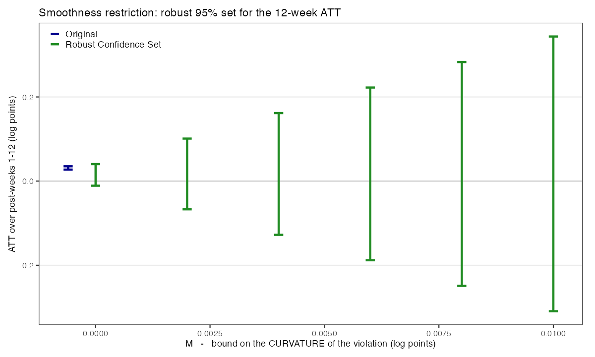

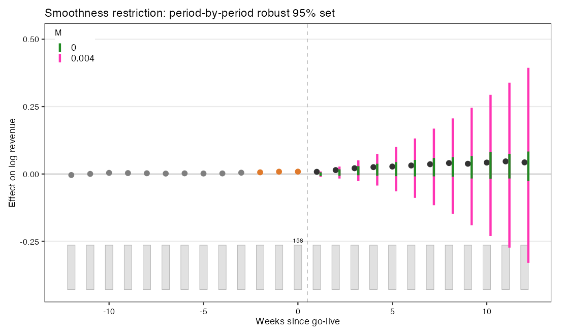
RM survives to 0.46. Smoothness dies at 0. Same panel, same fit, same estimand.

① \(M^{*}{=}\mathbf{0}\) — the strictest setting certifies nothing. The set is already [−1.10%, +4.04%] at \(M{=}0\): it contains zero, as do 12 of 12 weeks. The Original (navy, left) does not. \(\Delta^{SD}(0)\) says the violation is a straight line — not that it is absent — and a line fitted to a noisy pre-window and run out 12 weeks eats the whole effect.
② A step accumulates linearly; a bend accumulates quadratically. That is the only difference between the two restrictions — and it is worth 0.46 vs 0. Week 12 at \(M{=}0.004\): [−33%, +39%] for a +4% effect.  ⇒ THE RESTRICTION IS THE ASSUMPTION.

Test 4 of 4, and it closes the act — because it disagrees with Test 3, on the same data, and the disagreement IS the lesson.

THE IDEA. Delta-RM bounded how far the violation can STEP from one period to the next. Delta-SD bounds something different: how far it can BEND. Formally it caps the second difference — the change in the change. M = 0 means the second difference is exactly zero, which means the violation is exactly LINEAR: a straight line, extrapolated from the pre-period through the post-period. That sounds strict. It sounds, to most students, like the strictest thing you could possibly assume short of zero.

IT IS NOT, AND HERE IS THE RESULT: at M = 0 the robust confidence set for the twelve-week ATT is minus 1.10 to plus 4.04 percent. IT CONTAINS ZERO. The breakdown value M-star is ZERO. This restriction never certifies anything on this panel — not the average, and, look at the figure, not a single one of the twelve weeks. Twelve of twelve contain zero at M = 0.

WHY? Say this slowly, because it is the entire point. Delta-SD(0) does not say “there is no violation.” It says “the violation is a STRAIGHT LINE.” And which straight line? Any line consistent with the pre-period. The pre-period slope is estimated with noise; extrapolate a noisy slope twelve weeks forward and the range of lines you cannot rule out is enormous — easily big enough to contain the entire treatment effect. The restriction is not weak because the world is wild. It is weak because LINEAR EXTRAPOLATION IS EXPENSIVE, and it gets more expensive the further you go. Look at the pink intervals marching outward: at M = 0.004 — four tenths of a percentage point of curvature per week, which sounds like nothing — week 12’s set is minus 33 to plus 39 percent. For an effect of four percent. A bend accumulates QUADRATICALLY; a step only accumulates linearly. That is the whole difference between the two restrictions, and it is why they give opposite verdicts.

NOW LAND THE ACT. Same panel. Same fit. Same estimand. Same placebo. Two sensitivity analyses, both published, both principled, both implemented in the same function call — and one says your answer survives to M-bar 0.46 while the other says it never survived at all. Neither is wrong. They ASSUME DIFFERENT THINGS about the shape of what you cannot see. THE RESTRICTION IS THE ASSUMPTION — the inference-side twin of the estimation-side lesson from Act 2, where the PENALTY was the assumption. You do not escape assumptions by doing a sensitivity analysis. You relocate them, from the estimate into the robustness check, where they are harder to see and easier to shop for.

⚠️⚠️ READ THIS BEFORE YOU LECTURE. THE LEFT-HAND FIGURE ON THIS SLIDE IS THE REPAIRED ONE, AND THE CODE ON THE FACE WILL NOT REPRODUCE IT. A bare plot(s, type = “sens”, restrict = “sm”) in fect 2.4.5 comes out UNREADABLE. The professor’s call (2026-07-14) was to keep the slide clean — the figure and the substance on the face, the bug and its two-line fix in the SESSION NOTES only. So: DO NOT invite the room to run that line live, and if a student runs it and gets garbage, THEY DID NOTHING WRONG — send them to the notes. Everything below is your briefing, not slide content.

THE DEFECT — AND IT IS THE BEST BUG IN THE COURSE, which is why it is written up in full in the notes. Run plot(type = “sens”, restrict = “sm”) bare and you get garbage: what look like horizontal bars sprayed across the panel, and the “Original” band parked far off to the left. Earlier versions of these notes called it “transposed.” THAT WAS WRONG — I had diagnosed the symptom, not the cause, and I taught it wrong. Nothing is transposed. plot.fect builds aes(x = M) with a VERTICAL geom_errorbar, which is exactly right.

THE ACTUAL BUG IS TWO CONSTANTS HARDCODED IN X-AXIS UNITS. The errorbar’s cap width is fixed at 0.02, and the “Original” band is parked at x = -0.05. Now: M-bar is UNITLESS — a multiple of a ruler — so it always lands in [0, 1], where 0.02 is a 2% tick and -0.05 is just off to the left. Both constants are fine, forever, for the RM plot. BUT M IS IN THE OUTCOME’S OWN UNITS. On log revenue it spans 0.010. So the cap width is TWO HUNDRED PERCENT of the x-range, and Original sits five times the domain away. THE “HORIZONTAL BARS” ARE THE CAPS.

Two lines fix it — supply the missing M column so fect stops defaulting Original to -0.05, and scale the cap width to 0.02 x range(M) = 2e-4. That is the figure on the left of this slide, and it is worth pointing at: THE NAVY ORIGINAL EXCLUDES ZERO, AND THE VERY FIRST GREEN RUNG — AT M = 0, THE STRICTEST SETTING — ALREADY CROSSES IT. M-star = 0, visible.

AND HERE IS THE LESSON, WHICH IS NOT “DISTRUST THE PICTURE.” Rescale M by 100 — pretend the outcome were in percentage points — and the BARE call renders perfectly, with no patch at all. Same object, same numbers. So THIS BUG FIRES FOR SOME ANALYSTS AND NOT OTHERS, purely on a modelling choice that has nothing to do with it. A student who works in levels will never see it and will swear you are wrong. “IT WORKED FOR ME” PROVES NOTHING. When the figure and the object disagree, the object is the evidence — and you go read the source, because “the package is buggy” is not a diagnosis. (This is why the BROKEN CALL is not in Lab 3 and smoothness is NOT in A5: monkey-patching ggplot internals is not econometrics, and the bug would fire for the log students and not the levels students. But smoothness ITSELF is in Lab 3, as Test 4 — the lab draws it with plot(type = “sens_es”, restrict = “sm”), which is NOT affected by this bug and renders correctly. The lab warns them off the bare type = “sens” call in as many words: if they run it and get garbage, THEY DID NOTHING WRONG. So they compute M* = 0 themselves; we simply never ask them to patch a package, and we do not grade it in A5.)

ONE LAST HONESTY NOTE, AND IT IS INSTRUCTOR-ONLY — IT IS DELIBERATELY OFF BOTH FACES, so do not put it on the board unless a student asks. That +4.04% upper bound in the table is NOT a bound. It is 0.0403937 = 20 x SE, HonestDiD’s default SEARCH-GRID CEILING, and fect_sens() swallows HonestDiD’s own “CI is open at one of the endpoints” warning inside suppressWarnings(). The same ceiling flattens the top edge of Test 3’s left-hand figure — if a sharp student points at that dead-flat line and asks why a robust set stops widening, THAT is the answer, and it is the honest one: the upper edge is CENSORED, NOT BOUNDED. The interval is AT LEAST that wide; it is not EXACTLY that wide. Neither headline depends on it — Test 3’s M-bar-star and Test 4’s M-star both rest on the LOWER bounds, and those are clean (0 of 21 pinned). That is the only reason either number means anything. Full write-up in the session notes, and Lab 3 makes them compute the lid themselves.

Effect Heterogeneity

Same fit, two axes, two illusions

Why. Don’t aggregate at all — read the cells. Is the app hurting some stores?  plot(f, type = “box”)

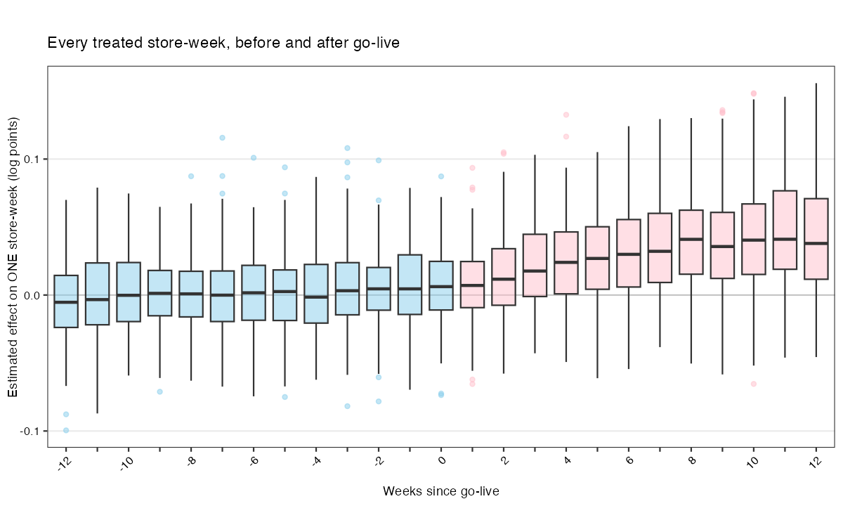
Looks like. 21.4% of the 1,896 post cells read negative (week 1: 38.6%) — “switch the app off in the stores it’s hurting.”

But. 48.0% of the blue cells do too — before go-live, no app. The unit FE is fitted on exactly those cells, so half must land below. The null is 50, not 0 — the losers are noise.

Read it as ⇒ the LOCATION, never a box. Pre: median ≈ 0. Post: it lifts and keeps lifting — +0.7% at launch → +4.1% by week 8. That climb is the effect. The width is error, not heterogeneity: it grows with the horizon (IQR 3.4 → 5.9 pp).

Why. Fine — aggregate, and ask when. Does the app work better in some weeks?  plot(f, type = “calendar”)

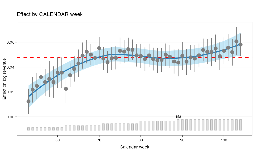
Looks like. +1.25% (wk 53) → +5.80% (wk 104) — a 4.8 pp swing, as large as the ATT itself. “It compounds: the app works better later in the year.”

But. No calendar is in it. Calendar time and tenure move together here: wk 53 is 40 stores at tenure 1, wk 104 is 158 at mean tenure 35. Rebuild the curve with no calendar term: inside the CI in 48 of 52 weeks. It tracks the grey bars — the rollout.

Read it as ⇒ DELIVERY, not modification. What the live fleet actually earned each week — true, and the right plot for that. High late because the fleet is mature. For “when does it work better?” you must hold tenure fixed; this plot cannot.

TWO COLUMNS, TWO TRAPS, ONE LESSON. Both are drawn from THE SAME FIT you have been staring at all hour. Neither trap is in the data. Both are in the AXIS you chose and the AGGREGATION you performed. Work left, then right; do not preview the right while you are on the left.

=== LEFT: THE CELL ===

LET THEM COMMIT FIRST. Point ONLY at the orange post-launch boxes. Four seconds is all an executive needs to reach “pull the app from the losers” — one store-week in five is in the red, and in the launch week it is nearly two in five. Ask the room for the decision. Take a show of hands. THEN move your hand left, to the blue.

The blue boxes are the SAME 158 stores in the 13 weeks BEFORE go-live — cells where no app exists. Forty-eight percent of them read negative. (Note the axis convention once, here, and it saves you later: fect’s event time 1 is the LAUNCH week; 0 is the last PRE week.)

Now say it PRECISELY, because the sloppy version is wrong and a sharp student will kill it. I am NOT telling you “the model thinks half the stores were harmed.” I am telling you that THE NULL VALUE OF THE STATISTIC IS 50, NOT ZERO.

Why 50? Because the treatment is ABSORBING. A treated store’s only untreated cells ARE its pre-launch cells — and the unit fixed effect for that store is fitted on exactly those cells. So the normal equations force its pre-period residuals to average EXACTLY ZERO. Half of them land below. That is an ALGEBRAIC IDENTITY, not a finding about coffee.

And it is not a property of IFEct either: run it with unit FE only, with two-way FE, with IFE at r = 1, and with a deliberately over-fitted IFE at r = 4 — four imputers of wildly different quality — and every one of them returns about fifty percent. SO “21% READ NEGATIVE” IS 21 MEASURED AGAINST 50, NOT AGAINST 0. It is a signal-to-noise ratio wearing a harm rate’s clothes.

And notice what I did NOT have to claim. I did NOT say the true effect in the pre-window is zero — THIS DECK ALREADY SHOWED YOU IT CANNOT CERTIFY THAT. The placebo fired at +0.78 pp, and the equivalence test could not certify the pre-window as small. I DON’T NEED IT. The 50% is a normal-equations identity: IT HOLDS WHATEVER THE TRUE PRE-EFFECT IS. That is why this argument is airtight and the seductive one is not.

Now read the BOXES, not the shares. Compare like with like — the last PRE week against the FIRST post week, one box against one box: the null box (week 0) has an interquartile range of 3.58 pp; the signal box (week 1), at the exact moment a manager makes the pull-the-app call, has 3.39 pp. THE NULL BOX IS TALLER THAN THE SIGNAL BOX. The signal is not merely small relative to the noise. AT LAUNCH IT IS INDISTINGUISHABLE FROM IT. (If you want the pooled number: all 2,054 pre cells together have an IQR of 3.94 pp — but that one is inflated by between-week variation, so DO NOT set it against a single week’s box. One box against one box. Same rule as everywhere else in this act.)

Say the prohibition BOTH WAYS, because someone will try to rescue the tails: the same imputation error that INVENTED harm here would just as happily HIDE real harm if it existed. YOU CANNOT READ THE TAILS FOR GOOD NEWS EITHER.

NOW THE CONSTRUCTIVE HALF, AND DO NOT SKIP IT — a refusal is not a reading. HOW SHOULD YOU READ THIS FIGURE? READ THE LOCATION. Not any one box, not the share negative, not the width: the LOCATION of the whole distribution. In the pre-window the median sits at ZERO — as it must. After launch it LIFTS AND KEEPS LIFTING: +0.7% in the launch week, +4.1% by week 8. THAT CLIMB IS THE EFFECT, and it is exactly the ramp the event study reports. The figure is not useless. It shows you the effect ARRIVING — you were just reading the wrong feature of it.

AND KILL ONE MORE TEMPTATION BEFORE IT STARTS, because the sharp student is already there: “fine, then the WIDTH is the heterogeneity — the post boxes are fatter, so stores must differ.” NO. The post boxes ARE fatter (IQR 3.4 pp in week 1, 5.9 pp by week 12) but that widening is IMPUTATION ERROR GROWING WITH THE HORIZON: post cells are OUT-OF-SAMPLE extrapolations, and the further you extrapolate the worse you predict. Worse, the pre-period boxes UNDERSTATE the noise floor, because those residuals are IN-SAMPLE — the unit FE is fitted on exactly them, so they are shrunk. So the pre spread is only a LOWER BOUND on the error. YOU CANNOT SUBTRACT THE VARIANCES AND CALL THE REMAINDER HETEROGENEITY. Not the level, not the tails, not the spread. THE ONLY THING THIS FIGURE LICENSES IS THE LOCATION.

=== RIGHT: THE AXIS ===

MOTIVATE IT AS THE OBVIOUS NEXT MOVE. “Fine — the cell is unreadable. So AGGREGATE. That is what aggregation is for.” And ask the most natural managerial question there is: does the app work better at some times than others? Season, macro, a competitor’s response, word-of-mouth building over the year. ONE ARGUMENT: type = “calendar”.

LET THEM COMMIT AGAIN. The path climbs from +1.25% in calendar week 53 to +5.80% in week 104. That is a 4.8-point swing — AS LARGE AS THE ENTIRE ATT. Every instinct in the room says: THE APP IS GETTING BETTER OVER TIME. Network effects. Word of mouth. The thing is compounding.

IT IS NOT. THERE IS NO CALENDAR IN THIS PLOT.

Point at the GREY BARS along the bottom — the treated count. THAT is the tell, and fect draws it for you. In calendar week 53 the treated set is FORTY stores, and every one of them is in its FIRST week of tenure. By week 104 it is ONE HUNDRED FIFTY-EIGHT stores at a mean tenure of THIRTY-FIVE weeks. And you have known since the ATT slide that THIS EFFECT RAMPS WITH TENURE: on this fit, +0.8% in week 1 and +4.3% by week 12.

So the calendar path is not measuring calendar. It is measuring THE RAMP, SAMPLED THROUGH A STAGGERED ROLLOUT. At every calendar week the treated set is a DIFFERENT MIXTURE OF TENURES, and the mixture matures as the rollout completes.

HERE IS THE PROOF, AND IT IS CHECKABLE. Take the event-time ramp — one number per tenure, nothing else — and average it over whichever tenures happen to be treated in each calendar week. NO CALENDAR TERM ANYWHERE IN THAT CALCULATION. It reproduces this path INSIDE THE ESTIMATE’S OWN 95% CONFIDENCE INTERVAL IN 48 OF THE 52 WEEKS. The mean gap is 0.52 pp against a mean standard error of 0.52 pp: the reconstruction sits inside the noise. A model that does not know what a calendar IS draws this curve.

AND THE DIPS PROVE IT TWICE. Look at weeks 62 and 71 — the curve drops 1.30 and 0.84 points, and each drop lands EXACTLY on a go-live wave: 28 new stores, then 29, each entering at tenure 1 with almost no effect yet, dragging the average DOWN. The rollout dilutes its own average. (Waves 4 and 5, at weeks 80 and 89, barely dent it — 0.05 and 0.08 pp — because by then they are a small addition to a large, mature treated base. Say so if asked; do not oversell a sawtooth that is only visible twice.)

⚠️ NOW BE FAIR TO THE PLOT, BECAUSE A GOOD STUDENT WILL DEFEND IT — AND THEY WILL BE RIGHT. “No calendar in it” is a statement about ONE estimand, not a verdict on the figure. This plot is the CORRECT answer to a genuinely different and genuinely managerial question: WHAT DID THE APP ACTUALLY DELIVER, WEEK BY WEEK, ACROSS THE FLEET THAT WAS LIVE AT THE TIME? That number really was +1.25% in week 53 and +5.80% in week 104. Nothing there is an artifact. If the CFO asks how much revenue the app added in Q4, THIS is the right plot and the event-study is the WRONG one — and the answer is high late precisely BECAUSE the fleet was mature, which is a fact about the business, not a bias.

So say it exactly: SAME NUMBERS, TWO ESTIMANDS. Read as DELIVERY, the curve is true. Read as “when does the app work BETTER” — as effect MODIFICATION by calendar time — it is empty, because a reconstruction with no calendar term reproduces it. AND NOTHING ON THE FACE OF THE PLOT TELLS YOU WHICH ONE YOU ASKED. That is the whole session in one figure, and it is why the slide says THE AXIS IS THE QUESTION rather than “this plot is junk.” Do not let them leave thinking fect’s plots are junk.

⚠️ TRACE NOTE, SO A SHARP STUDENT DOES NOT CATCH YOU: the red dashed line on this figure is +4.78%, not the +4.76% headline. Both are correct. +4.76% is the CV-SELECTED fit; this figure is drawn from the FIXED-r refit, and the line it draws is THAT object’s own ATT. The ramp endpoints shift the same way (+0.75/+4.25 on the CV-selected fit, +0.76/+4.28 here) — which is why slide 16 says +0.7% and I just said +0.8%. A NUMBER IS A PROPERTY OF A FIT. If nobody asks, do not raise it.

FORWARD POINTER, and it is worth planting out loud: “calendar week is confounded with tenure in a staggered absorbing rollout.” TWO SLIDES FROM NOW fect will happily draw a CATT curve against temp_c — WEATHER, a covariate the treatment does not move (p = 0.21). Its sin is not endogeneity. Its sin is that 95% of temp_c’s LEVEL is the calendar week (on the treated cells the plot uses) — the very axis you just watched lie. SAME CONFOUND, SECOND COSTUME. If you plant it here, that slide lands in ten seconds instead of two minutes.

INSTRUCTOR-ONLY, and it is an oracle so it stays off the face: the generator has NO calendar term at all — tau = tau_max × (1 − exp(−rate × weeks_since)), a function of TENURE and the store’s ceiling, full stop. The reconstruction above found that WITHOUT BEING TOLD, from the panel alone. Visible to you only because this is simulated; the argument on the slide does not need it, which is exactly why the slide does not use it.

=== LAND BOTH ===

Same fit. Same cells. Two axes, two illusions. The cell said “one in five is hurt” and its null was 50. The calendar said “it doubles across the year” and it had no calendar in it. NEITHER NUMBER IS WRONG. Both READINGS are — and the error is not in the data, it is in what you aggregated over and what you plotted against. THE AGGREGATION IS THE QUESTION. That is the same blade as S09, and it is the one A5 is graded on.

Now say what this slide does NOT say, because this is the scoping sentence and it is not optional: THIS IS A PROHIBITION ON READING A CELL AND ON READING AN UNCHOSEN AXIS. IT IS NOT A DENIAL THAT HETEROGENEITY EXISTS. In four minutes I will split these same stores three ways and the spread will be five points with standard errors of a fifth of a point. Heterogeneity is REAL. Cells are NOT READABLE. Both are true, and ONLY A DEFENSIBLE AGGREGATION BUYS THE DIFFERENCE.

S09 ANCHOR, if they push: in S09 there WAS a test that the heterogeneity is real — the BLP of the orthogonal score. A cell effect in a factor-imputation model has NO orthogonal score. There is no test. Only a refusal, and then an aggregation.

FOOTNOTE, if asked: the ~50% identity is exact over the FULL pre-window. On the last-13-weeks window shown here, an imputer that does not absorb the common time trend (unit-FE only) drifts to about 34%, because the late pre-weeks sit above the store’s own pre-mean. Two-way FE and both IFE fits all land at 48-50%. The identity needs the model to absorb the trend; every model you would actually use does.

Route 1 — group=: split the panel, and let fect refit

A discrete split needs no covariate in the model at all — there is no slope for the unit FE to absorb. fect refits each group and bootstraps it.

df$urban_tertile <- cut(u,
  quantile(u, c(0, 1/3, 2/3, 1)),
  include.lowest = TRUE,
  labels = c("Low urban",
             "Mid urban",
             "High urban"))

fg <- fect(log_rev ~ app_live,
  data = df,
  index = c("sid","week"),
  method = "ife", r = 1,
  force = "two-way", se = TRUE,
  group = "urban_tertile")

fg$est.group.att

group	ATT	S.E.
Low	+1.60%	0.21 pp
Mid	+4.61%	0.21 pp
High	+7.34%	0.21 pp

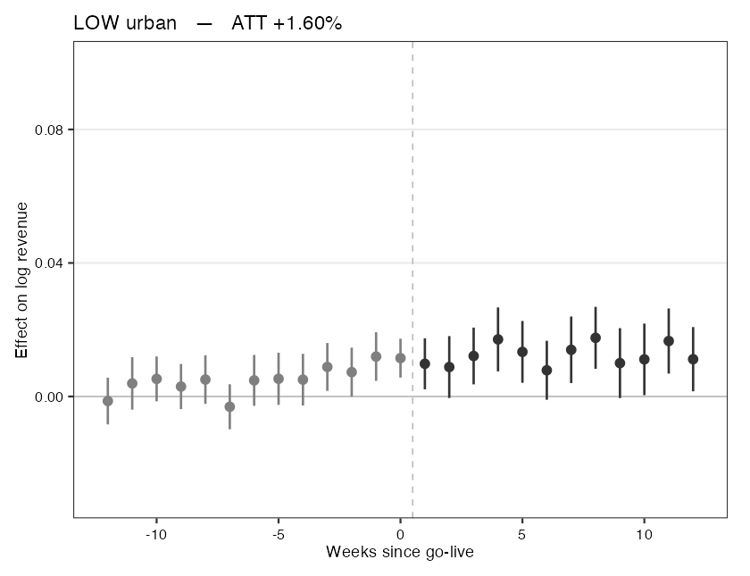
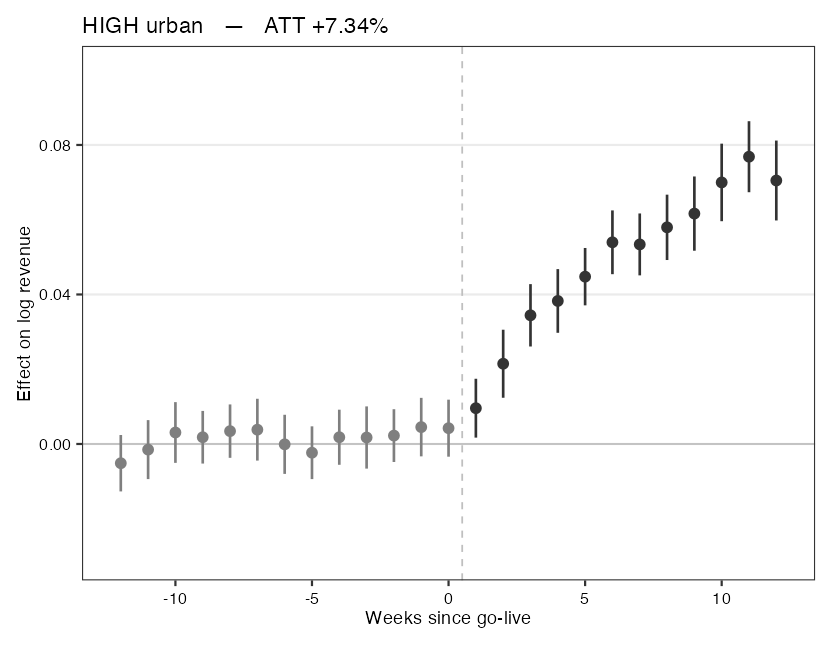
Read it as ⇒ same axis, two panels — the heterogeneity is the gap between them. Low is flat at ~+1%; High ramps to ~+7%. A 5.75-point spread, SE 0.21 pp, intervals nowhere near touching. This is the aggregation that buys back what the cell forbade — and its band is a real bootstrap.

ROUTE 1 OF 2. The question is now the one every manager asks: DOES THE APP WORK BETTER IN URBAN STORES? And the answer requires a method, not a plot.

START WITH THE OBSTACLE, because it is the reason there are two routes. The moderator you want is urban_share — a STORE ATTRIBUTE. It never changes. Put it in the outcome model and the UNIT FIXED EFFECT ABSORBS IT ENTIRELY: there is nothing left for a coefficient to identify. fect does not fail quietly, it refuses at FIT time and names your variable: “Variable urban_share is unit-invariant. Try to remove it.” It refuses all six BeanBuzz store attributes this way — market_size, urban_share, drive_thru, seats, baseline_tier, competitor_density. Every moderator a manager cares about. The within-store sd of every one of them is EXACTLY ZERO.

⚠️ READ THE CODE ON THE FACE BEFORE A STUDENT DOES. The tertiles are QUANTILE tertiles — quantile(u, c(0, 1/3, 2/3, 1)) — i.e. EQUAL COUNTS (85 / 72 / 76 stores). They are NOT cut(urban_share, 3), which makes equal-WIDTH bins (85 / 55 / 93) and puts 17 of the 233 stores in a different tertile. That is not cosmetic: equal-width returns Mid +4.30% and High +6.97% (spread 5.37 pp) instead of the +4.61% / +7.34% (spread 5.75 pp) in the table on this slide. The face carried the equal-width call for a while and NOBODY CAUGHT IT, because LOW URBAN COMES OUT IDENTICAL EITHER WAY (+1.60%) — the one group everyone checks first. Fixed 2026-07-14; the lab uses the quantile convention and says so in as many words.

NOW THE KEY INSIGHT, AND IT IS ONE LINE: group= DOES NOT PUT THE COVARIATE IN THE MODEL AT ALL. It SPLITS THE PANEL. A discrete split has no slope, so there is nothing for the fixed effect to eat. fect simply refits the whole estimator inside each group and bootstraps each one. The constraint evaporates — not because we were clever, but because we asked a different question.

READ THE TWO PANELS. And point at the y-axis FIRST, because this is the only reason the pair works: I PINNED THEM TO THE SAME SCALE. fect auto-scales each plot to its own data, and if you let it, Low urban and High urban render as visually IDENTICAL ramps on different axes — the picture would say “no heterogeneity” while the numbers screamed the opposite. Same axis. Now look: LOW IS FLAT AT ABOUT ONE PERCENT. HIGH RAMPS TO SEVEN. That gap IS the heterogeneity, and you can see it from the back of the room.

THE NUMBERS: +1.60, +4.61, +7.34 percent. A 5.75-POINT SPREAD, with standard errors of 0.21 points — intervals nowhere near touching. And say what this is, because the first slide of this act forbade it: A CELL IS UNREADABLE. A GROUP IS NOT. Only aggregation buys the difference, and here is the aggregation, with a REAL BOOTSTRAP BAND under it.

TWO HONEST CAVEATS, one sentence each, and do not skip them.

FIRST — COMPOSITION, and catch it with your own rule from the calendar slide. est.group.att averages ALL post weeks. The effect RAMPS. And the low-urban stores went live about NINE WEEKS LATER than the rest — mean treated tenure 18.8 vs 26.2 vs 27.9 weeks. So the three groups are averaged over windows of DIFFERENT LENGTHS ON A GROWING PATH. Put all three on a common 12-week horizon and the spread is +1.25, +2.92, +4.94: THREE POINT SIX NINE, NOT FIVE POINT SEVEN FIVE. THIRTY-SIX PERCENT OF YOUR HEADLINE MODERATION IS ROLLOUT TIMING. The moderation SURVIVES. The NUMBER does not.

SECOND — THE PLACEBO INSIDE EACH GROUP. Run the placebo test within group and Low urban’s pre-period fires: +1.29 points, p = 0.000, against a group ATT of +1.60. Its placebo is EIGHTY PERCENT OF ITS OWN ESTIMATE. High urban’s placebo sits on zero. So the ONE GROUP A BOARD WOULD DEPRIORITISE IS THE ONE GROUP WHOSE NUMBER IT CANNOT USE — and note the asymmetry, because it is the S12 refrain: THE AUDIT CAN CONVICT, IT CAN NEVER ACQUIT. High urban passing its placebo does not make High urban’s number true.

Route 2 — type="hte": build the covariate

type="hte" smooths the cell effect against a covariate’s raw level — so the covariate must be in the model, and it must clear four hurdles:

it must…	or else — and what it kills
1. vary within store	the unit FE eats it → “unit-invariant”. Kills all 6 store attributes — incl. urban_share
2. be nonzero on the untreated cells	fect fits Y(0) only there. urban_share × app_live is identically 0 → collinear. The moderator is only “on” where fect refuses to look.
3. not be moved by the treatment	else it is a bad control. Kills mktg_spend: +€251, t = 130
4. not be a clock	else you are plotting the tenure ramp. Kills temp_c (95% week) and footfall_index (88%)

No raw covariate in the panel clears all four. So build one:

df$urban_x_week <- df$urban_share * df$week

fuw <- fect(log_rev ~ app_live + urban_x_week,
   data = df, index = c("sid","week"), method = "ife",
   r = 1, force = "two-way", se = TRUE)

plot(fuw, type = "hte", covariate = "urban_x_week")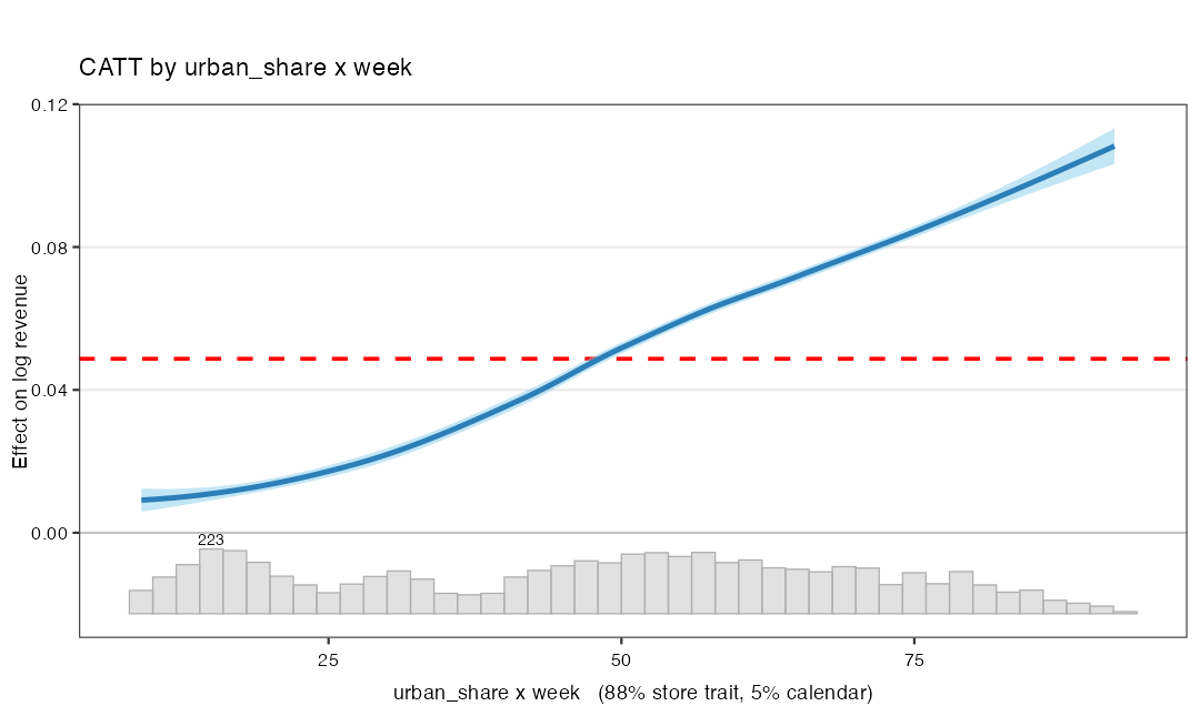

It clears all four. Within-store sd 15.8 ①; sd 17.5 on the untreated cells ②; deterministic in (store, week) — the treatment cannot move it ③; and on the treated cells it is 88% store trait, 5% calendar ④ (the treated calendar spans 2×; urban_share spans 9× — the product is urbanity, not time).

Read it as ⇒ a continuous gradient (+0.9% → +10.8%) that agrees with group= — at two prices: the covariate is in the model, so it moved the estimator (+4.78% → +4.87%); and the ribbon is a loess SE over 5,606 cells treated as independent — it never touches the bootstrap, even here with se = TRUE.

⇒ group= GIVES A BAND.  type="hte" GIVES A SHAPE.

ROUTE 2 OF 2, and it is the one everybody reaches for first — plot(type = “hte”, covariate = “urban_share”) — so let us find out exactly what it costs.

WHAT THE PLOT ACTUALLY DOES, because it is not what people assume: it takes the CELL EFFECTS, takes the covariate’s RAW LEVEL at each of those cells, and LOESS-SMOOTHS one against the other. That is all. It is a kernel-weighted version of group= with a continuous axis. And it demands that the covariate be IN THE OUTCOME MODEL.

WALK THE FOUR HURDLES. Do not rush this — the table is the slide.

ONE: IT MUST VARY WITHIN STORE. The unit FE absorbs anything constant, so fect refuses at fit time. That kills all SIX store attributes — every moderator anyone cares about, urban_share included.

TWO, AND THIS IS THE DEEP ONE, so slow down. The obvious fix is: “fine, MAKE it time-varying — interact it with the treatment.” urban_share TIMES app_live. It varies within store now. IT DOES NOT WORK, and the error message is not the interesting part; the REASON is. FECT FITS Y(0) ON THE UNTREATED CELLS ONLY. That is not a quirk, THAT IS THE WHOLE IMPUTATION IDEA — fit the white cells, predict the grey ones. And urban_share times app_live is IDENTICALLY ZERO on every untreated cell. Sd of zero point zero zero zero. It is collinear with the fixed effects and feols aborts. SAY THE SENTENCE: A TREATMENT-EFFECT MODERATOR IS, BY CONSTRUCTION, ONLY “ON” INSIDE THE VERY BLOCK FECT IS REFUSING TO LOOK AT. You cannot teach the imputation model about the moderator using the cells it has sworn off.

THREE: THE TREATMENT MUST NOT MOVE IT. mktg_spend is time-varying and fect takes it happily — and it is a BAD CONTROL. Regress it on the treatment with store and week FE: PLUS 251 EUROS, t of 130. Your treatment moves your control, therefore it is not a control. It also moved the headline.

FOUR: THE AXIS MUST NOT BE A CLOCK. This is the calendar lesson, arriving for the second time. type=“hte” smooths against the covariate’s LEVEL — and if that level is mostly “which week is it”, you are plotting the TENURE RAMP wearing a covariate’s name. temp_c is 95% calendar week. footfall_index is 88%. Both fect will draw. Both are the ramp in disguise.

SO: NO RAW COVARIATE IN THIS PANEL CLEARS ALL FOUR. That is not bad luck — it is structural, and it is worth naming: the covariates fect WILL draw are exactly the time-varying ones, and in an absorbing rollout the time-varying ones are exactly the ones your treatment may have MOVED, or the ones that are secretly a clock. THE API’S CONSTRAINT SELECTS FOR BAD CONTROLS.

SO BUILD ONE. urban_share TIMES WEEK. And check it against all four, out loud: within-store sd 15.8, so fect accepts it. Nonzero on the UNTREATED cells — sd 17.5 — so fect can actually fit it, which is where the app_live interaction died. It is DETERMINISTIC in store and week, so the treatment CANNOT move it — hurdle three is not passed, it is UNPASSABLE-BY-CONSTRUCTION. And hurdle four, the one I got wrong the first time: on the TREATED cells — the only cells this plot uses — it is 88% STORE TRAIT and 5% CALENDAR. Why? Because among treated cells the calendar only spans weeks 53 to 104, a factor of two, while urban_share spans 0.1 to 0.9, a factor of NINE. THE PRODUCT IS URBANITY, NOT TIME.

NOW READ THE CURVE. It sweeps from about +1% to nearly +11%, monotone, and it AGREES with the tertiles — a continuous gradient where group= could only give you three rungs. That is the payoff, and it is real.

AND NOW THE TWO PRICES, because this is the slide’s actual lesson and it is a trade, not a winner.

PRICE ONE: the covariate is IN THE MODEL. So it changed the Y(0) imputation, and IT MOVED THE ESTIMATOR — 4.78 to 4.87 percent. group= never touches the estimator; it only splits the sample. You bought a nicer picture with a different headline.

PRICE TWO, AND IT IS THE ONE THAT MATTERS: THAT RIBBON IS NOT AN INFERENCE BAND. Go read the source. It is qt(0.975, df) times the LOESS standard error, computed over 5,606 cell effects TREATED AS INDEPENDENT OBSERVATIONS. It does not propagate the imputation uncertainty. It does not cluster by store or by market. AND — this is the part that surprised me — IT NEVER TOUCHES THE BOOTSTRAP, EVEN ON THIS FIT, WHERE se = TRUE AND 200 BOOTSTRAP DRAWS ARE SITTING IN THE OBJECT. It ignores them. So a tight ribbon here means nothing except “loess had a lot of points.”

LAND IT: group= GIVES YOU A BAND. type=“hte” GIVES YOU A SHAPE. Use the shape to SEE the gradient; use the band to DEFEND it. And never read a package’s willingness to draw a plot as a licence to interpret it.

The completed assumption ledger

Every estimator in Part V assumed treatment was not set by past outcomes — strict exogeneity. Unpacked, it forbids feedback, lagged-outcome dependence, and carryover (Liu, Wang, and Xu 2024; Imai and Kim 2019).

Row	Assumption	Buys	Costs
0	Strict exogeneity	licenses all of Part V	no feedback / LDV / carryover
1 · S10	Parallel trends	cheap, additive, whole cohort	blind to a unit×time factor
2 · S11	Hull + loadings	a counterfactual at N=1	hull, non-overfit fit, weak inference
3 · S12	Low rank	recovers the latent factor	rank tuning; restriction choice; bands are frontier

If treatment was set by outcomes, none of this holds — you leave Part V for g-methods (MSM, PanelMatch). (Imai and Kim 2019)

The penalty, then the restriction

Every rung fills the same blank under a different assumption, and they diverge only on the grey cells you can’t check. Estimation: the penalty is the assumption. Inference: the restriction is the assumption. A point estimate without a defensible assumption and a band is not a finding.

Close the assumption ledger that has accumulated across the whole part, and name the one assumption beneath all of it. Every Part V estimator — DiD, synthetic control, interactive fixed effects, matrix completion — quietly assumed STRICT EXOGENEITY: treatment was not driven by the outcome’s own past. Following Liu-Wang-Xu and Imai-Kim, it forbids feedback (a revenue dip triggering the launch), lagged-dependent-variable dynamics, and carryover. In BeanBuzz the waves were scheduled at baseline on market size, not in response to revenue, so it is plausible — but if managers had launched precisely where revenue had just dipped, every number would be biased. Walk the completed ledger row by row — the single artifact that ties S10, S11, S12 together. Row 0, strict exogeneity, licenses the enterprise. Row 1, parallel trends (S10): a cheap additive estimator, blind to a unit×time factor. Row 2, hull + loadings (S11): a counterfactual for a single unit, but needs the treated unit inside the donor hull with a non-overfit pre-fit and pays with weak inference. Row 3, low rank (S12): recovers the latent factor, but must tune the rank and its bands are a frontier. This ledger IS the A5 memo skeleton: name the assumption your estimator buys, and argue it is plausible here. And the escape hatch: if strict exogeneity fails, you have left the parallel-trends world for g-methods — a different course, and the boundary of everything Part V taught.

The closing callout is the discipline that makes the whole ledger useful rather than merely tidy, and it is the last thing they carry out the door. On the OBSERVED cells every method fits well — that is what fitting does. They only DISAGREE on the grey cells you can never verify, and there the entire +4.2%-vs-+4.9% gap is the penalty’s assumption, not the data. So the only honest basis for choosing is which assumption you can DEFEND in this business context — is parallel trends plausible here, or is there obviously a seasonality factor? — not which estimate has the prettiest standard error. Same lesson as Part IV’s “pick the identification strategy, not the significant coefficient”: this is the sentence A5 is testing.

AND NOW THE SECOND LAYER, which today added and which the ledger’s “restriction choice” cost now records. The ledger has always priced the ESTIMATION assumption. The sensitivity act showed there is another one underneath it. The +4.2%-vs-+4.9% gap on the grey cells is the PENALTY’s assumption. The [+1.6, +2.9] vs [−1.1, +4.0] gap — on the SAME grey cells, from the SAME fit — is the RESTRICTION’s. Relative magnitudes and smoothness were handed IDENTICAL DATA and returned OPPOSITE VERDICTS: RM at its zero excludes zero, SD at its zero contains it. They disagree because they encode different beliefs about what the unobserved violation IS — RM bounds how much it can CHANGE, SD bounds how much it can CURVE — and both of them have a setting called “zero” that assumes an entirely different thing.

And now the sentence that matters, and note what it does NOT do: IT DOES NOT TELL YOU WHICH ONE WAS RIGHT. You cannot know that. The violation lives on the grey cells, and the grey cells are the ones you never see — that is the definition of the problem, and no sweep, no package and no amount of bootstrapping will hand it back to you. What you CAN do is exactly three things, and they are what A5 is graded on: NAME THE SHAPE you expect the leftover to have and say why it is plausible in THIS business; SHOW WHAT IT COSTS by reporting the breakdown value WITH THE UNITS IT IS DENOMINATED IN; and if you cannot name the shape, REPORT BOTH RESTRICTIONS and let the reader see them disagree.

That is the whole discipline, in both layers. In estimation, the penalty is the assumption. In inference, THE RESTRICTION IS THE ASSUMPTION. Neither is ever tested. Both are asserted, and the only honest thing you can do with an assertion is to declare it in advance, defend it on the business, and price it out loud.

References

Athey, Susan, Mohsen Bayati, Nikolay Doudchenko, Guido Imbens, and Khashayar Khosravi. 2021. “Matrix Completion Methods for Causal Panel Data Models.” Journal of the American Statistical Association 116 (536): 1716–30. https://doi.org/10.1080/01621459.2021.1891924.

Athey, Susan, and Guido W. Imbens. 2017. “The State of Applied Econometrics: Causality and Policy Evaluation.” Journal of Economic Perspectives 31 (2): 3–32. https://doi.org/10.1257/jep.31.2.3.

Borusyak, Kirill, Xavier Jaravel, and Jann Spiess. 2024. “Revisiting Event-Study Designs: Robust and Efficient Estimation.” Review of Economic Studies 91 (6): 3253–85. https://doi.org/10.1093/restud/rdae007.

Imai, Kosuke, and In Song Kim. 2019. “When Should We Use Unit Fixed Effects Regression Models for Causal Inference with Longitudinal Data?” American Journal of Political Science 63 (2): 467–90. https://doi.org/10.1111/ajps.12417.

Liu, Licheng, Ye Wang, and Yiqing Xu. 2024. “A Practical Guide to Counterfactual Estimators for Causal Inference with Time-Series Cross-Sectional Data.” American Journal of Political Science 68 (1): 160–76. https://doi.org/10.1111/ajps.12723.

Xu, Yiqing. 2017. “Generalized Synthetic Control Method: Causal Inference with Interactive Fixed Effects Models.” Political Analysis 25 (1): 57–76. https://doi.org/10.1017/pan.2016.2.

Thank you for your attention!
	www.startupengineer.io/team/ihl/ christoph-ihl christophihl