15  Session 10: Difference-in-Differences

15.1 Lecture Slides

Open slides in new tab | Download as PDF

15.2 Overview

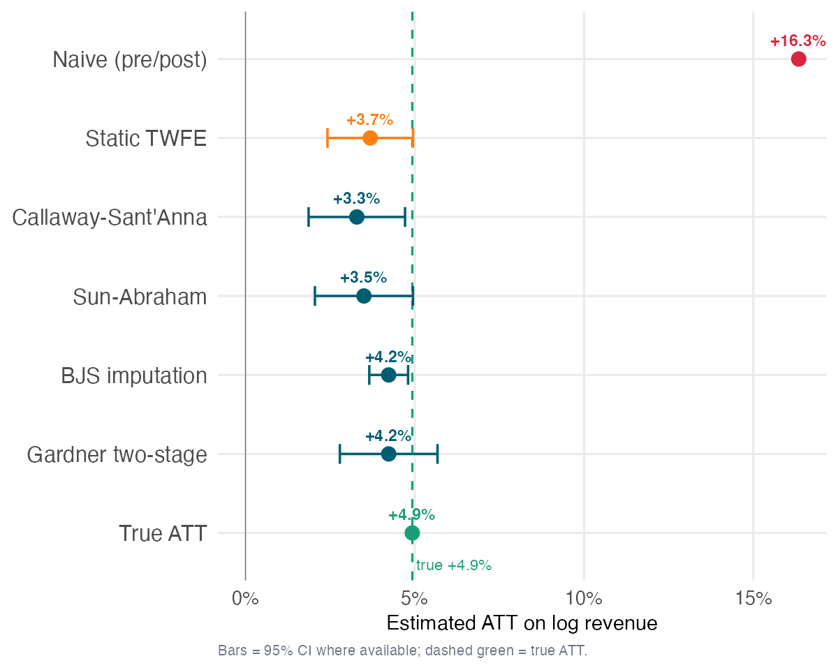
BeanBuzz’s CFO has a chart that looks like a triumph: every market that launched the loyalty app saw revenue climb, and a naive before/after on the launched markets puts the lift at a career-making +16.3%. The chart is a trap — a treated-only before/after books everything else that moved between the two windows (a secular uptrend, the winter-peaking coffee seasonality), so the +16.3% mostly measures the common time movement every market would have seen anyway — +11.4pp of pure time on top of the true +4.9%. This session is Part V’s first answer to the recurring problem: we never see what a treated market would have done without the app — the missing \(Y(0)\) — so we have to impute it. Difference-in-differences fills that blank with the cheapest, oldest assumption, an additive unit + time model that is exactly parallel trends: subtract the common time movement a comparable market would have had anyway, and what survives is the app’s effect. The headline arc carries that correction through a family of estimators — naive +16.3% (mostly time) → static TWFE +3.7% (correct in direction but biased downward by “forbidden” comparisons under staggered timing) → a heterogeneity-robust family (Callaway-Sant’Anna, Sun-Abraham, Borusyak, Gardner) that converges tightly to +3.3–4.2% — against a true ATT of +4.9%. The robust family does not recover the truth; it lands systematically just below, and that residual gap is a deliberate clue (an omitted regional-economy factor the additive model cannot represent) that motivates synthetic control (S11) and counterfactual imputation (S12). Two through-lines tie the session to its neighbours: back to S09, the doubly-robust ATT inside Callaway-Sant’Anna is the same AIPW score — now computed on first-differenced outcomes (“AIPW-on-differences”), so DML-DiD is the orthogonal score we already know; forward to S11, that residual gap is the cue to corroborate the DiD lens with synthetic control — a method that does not lean on parallel trends — precisely for the single-flagship cases (a lone store like Northgate) where a cohort-based DiD has no comparison pool to lean on.

Learning objectives. By the end of this session you will be able to:

• Diagnose why a naive pre/post comparison (+16.3%) and static TWFE (+3.7%) both diverge from the true ATT (+4.9%) — the naive books common time movements, static TWFE the negative-weight pathology — and why a non-random rollout (biggest markets first) requires parallel trends rather than any control.
• Justify parallel trends as the identifying assumption that imputes \(Y(0)\) via additive unit + time effects, and read an event study correctly — distinguishing a flat pre-trend (a diagnostic) from a proof of parallel trends (impossible).
• Estimate a heterogeneity-robust ATT using Callaway-Sant’Anna ATT(g,t) as the spine, and demonstrate convergence of CS / Sun-Abraham / Borusyak / Gardner to the same target — in both R (did) and Python (differences), reproducing the exact-parity +3.3%.
• Run and interpret a HonestDiD sensitivity analysis: compute the breakdown value — how large a parallel-trends violation, relative to the worst pre-period wobble, overturns the conclusion — and report a band, not a point.
• Connect the Sant’Anna-Zhao doubly-robust DiD score to the S09 AIPW machinery (“AIPW-on-differences”), and articulate when the DiD lens fails and a single-flagship synthetic-control lens is the right tool — setting up S11.

15.3 Lecture Notes

15.3.1 Act 1 — Introduction: the pre/post trap

15.3.1.1 The CFO’s memo and the pre/post trap

15.3.1.2 A rollout that looks like a triumph

BeanBuzz is a coffee chain rolling its loyalty app out across 40 regional markets in five staggered waves. The CFO’s slide is unambiguous: average weekly revenue in each launched market climbs after go-live, and the memo asks one operational question — accelerate the remaining waves? The seductive way to answer it is a before/after comparison on the treated markets: take app-era revenue minus the pre-app baseline, pooled across all launched stores. On BeanBuzz that pre/post difference in log revenue is

\[\widehat{\text{naive}} \;=\; \bar Y^{\text{treated}}_{\text{post}} - \bar Y^{\text{treated}}_{\text{pre}} \;=\; +16.3\%.\]

Sixteen percent on revenue is a career-making number. It is also wrong, and the rest of the session is why. The error is the oldest one in causal inference: a pre/post comparison attributes to the app everything else that changed between the two periods — the winter seasonality and the secular macro trend that lifts every market, launched or not. There is no control for “what would have happened anyway.”

15.3.1.3 One sign convention, stated once

Throughout, the outcome \(Y\) is log weekly revenue per store, so every estimate reads as a percentage change, and the app’s true effect is positive — it adds revenue. This is the opposite of the prior assignment’s cost outcome, where a lower number was the win. Keep the direction straight: here bigger is better, the app helps, “biased toward zero” means biased downward from +4.9%, and when HonestDiD asks whether the effect “survives,” it is the positive sign and significance being stress-tested.

15.3.1.4 The confound, made visible

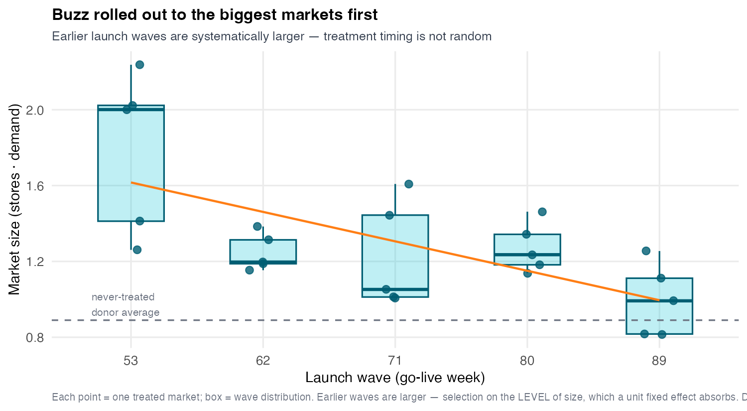
Plot each market’s launch wave against its size and the pattern is stark (Figure 15.1): the earliest waves — weeks 53 and 62 — were the biggest markets; later waves were smaller. The rollout selected on size, a level — a perfectly rational product-management heuristic, but not what inflates the naive: a market’s size sits in both the pre and post windows, so it cancels in a within-market before/after (the +16.3% is time, not selection — see above). What the non-random rollout does tell you is which control is legitimate. Treated and never-treated markets differ in level, so you need a control whose trend the treated markets share — exactly what parallel trends buys, with a unit fixed effect removing the size gap for free. The bias a DiD cannot survive is selection on the trend — rolling out precisely where growth was already accelerating — because no unit fixed effect can subtract a slope. Here selection was on level, not trend, so parallel trends is plausible; that is the assumption the session leans on, and the one Assignment V makes you stress-test when a cohort violates it.

Figure 15.1: Each treated market’s launch wave against its market size (BeanBuzz). Markets that launched earliest (waves 1 and 2, weeks 53 and 62) are the largest; later waves are smaller, and the never-treated donors are smaller still. The rollout selected on the level of size — which a unit fixed effect absorbs — not on the outcome trend. The naive +16.3% is inflated by common time movements (a secular uptrend plus winter seasonality), not by this size gap, which cancels in a within-market comparison.

15.3.1.5 This session in one line

The whole method, compressed: subtract the common time trend a comparable market would have had anyway — what’s left is the app’s effect. That subtraction is an imputation of the missing \(Y(0)\): we fill each treated market’s unseen no-app path using markets that didn’t (yet) get the app. This is the Part V spine — impute the missing \(Y(0)\) under escalating assumptions. S10 uses additive unit + time effects, which is the parallel-trends assumption; S11 relaxes it (synthetic control); S12 generalizes it (counterfactual imputation). Hold the image of a spreadsheet with a blanked-out rectangle (the treated-and-post cells); the next three sessions fill that rectangle under progressively weaker assumptions, and today’s is the boldest-but-simplest.

15.3.2 Act 2 — The basic 2×2 model

15.3.2.1 The canonical 2×2 and the DiD estimand

15.3.2.2 Two markets, four numbers

Build the intuition on the smallest possible case before scaling to the staggered rollout. Take one wave-1 (week-53) market, one never-treated donor market, and two periods — pre-launch and post-launch (Figure 15.2). Index both to 100 in the pre-period. That gives four cell means, and the entire DiD method is an arithmetic operation on those four numbers; everything more elaborate is built by aggregating cases exactly like this one.

Figure 15.2: The canonical 2×2: a wave-1 treated market and a never-treated donor, each at a pre- and post-launch period, indexed to 100 pre-period. The four cell means form a parallelogram; the gap between the treated market’s actual post value and the dashed counterfactual (the control’s change applied to the treated baseline) is the difference-in-differences, +5.2% — the clean early-cohort effect, far below the naive +16.3%.

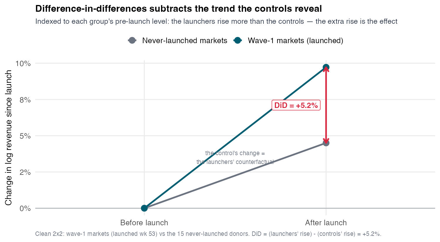
Look only at the treated market: its revenue rises from pre to post. That jump bundles two movements you cannot separate from one market — the app’s effect (what we want) and everything else that changed between the periods (the winter seasonality and the macro trend that lifted every market). The single-market before/after is the +16.3% mistake in miniature.

15.3.2.3 The control is the borrowed counterfactual

The never-treated donor got no app, so its entire pre-to-post change is pure time — seasonality plus macro plus trend, with no treatment component. DiD’s identifying move is to borrow that change: assume the treated market would have moved by the same amount absent the app, so the control’s change is our estimate of the treated market’s unseen no-app change. This is the imputation of \(Y(0)\) made concrete — the control’s \(\Delta\) is the treated market’s missing \(Y(0)\) trend. Crucially, the assumption is about the change (the trend), not the level: the two markets can sit at very different revenue levels and DiD is still valid, as long as they would have moved in parallel.

The estimator subtracts the control’s change from the treated market’s change:

\[\widehat{\text{DiD}} \;=\; \underbrace{\big(\bar Y^{\text{treat}}_{\text{post}} - \bar Y^{\text{treat}}_{\text{pre}}\big)}_{\text{treated jump (effect + time)}} \;-\; \underbrace{\big(\bar Y^{\text{ctrl}}_{\text{post}} - \bar Y^{\text{ctrl}}_{\text{pre}}\big)}_{\text{time alone (the imputed } Y(0) \text{ trend)}}. \tag{15.1}\]

The second term is the imputed \(Y(0)\) trend; what survives the subtraction is the app’s effect, free of the common time movement. On the wave-1 market versus the never-treated donor, this 2×2 gives DiD = +5.2% — roughly two-thirds of the apparent +16.3% was the common time movement (trend + seasonality). Stress that +5.2% is the wave-1 number (early cohorts, biggest markets), a clean building block, not the portfolio-wide ATT the robust estimators will later pin near +3–4%.

15.3.2.4 The estimand: the ATT, not the ATE

Name what that number estimates. DiD targets the average treatment effect on the treated (ATT), \[\tau_{\text{ATT}} \;=\; \mathbb{E}\!\left[\,Y_{it}(1) - Y_{it}(0) \mid \text{treated, post}\,\right], \tag{15.2}\] the effect of the app on the markets that actually launched, over their post-launch periods — not the effect on a random market (the ATE). The distinction is not pedantic: it is why DiD needs less than randomization. The ATE would require full unconfoundedness, \(\{Y(0),Y(1)\}\perp D\) — treated and control comparable on both potential outcomes. DiD needs only the treated group’s counterfactual \(Y(0)\) path to be borrowable — a one-sided condition on \(Y(0)\) alone, which is exactly parallel trends (Equation 15.5). This is the unconfoundedness scaffolding of S06–S09, moved from the level of \(Y\) to its change: DiD is ignorability-in-differences. The narrower estimand — the treated, not everyone — is the price of the weaker assumption. The cohort-time object the robust estimators actually compute, \(\text{ATT}(g,t)\) (Equation 15.8), is this same estimand refined to one cohort and period.

15.3.2.5 With two periods, TWFE just recomputes the 2×2

The regression form of the same arithmetic is the two-way fixed-effects model:

\[Y_{it} \;=\; \alpha_i \;+\; \lambda_t \;+\; \tau\,D_{it} \;+\; \varepsilon_{it}, \tag{15.3}\]

where \(\alpha_i\) is the market fixed effect (sweeping out the level), \(\lambda_t\) is the period fixed effect (sweeping out the common time movement), and \(D_{it}\) is the treatment indicator. With one treated group and two periods, \(\hat\tau\) equals the hand-computed 2×2 of Equation 15.1 exactly. This equivalence is genuinely reassuring in the canonical case and is why TWFE became the default reflex for panel data. But plant the time bomb now: the equivalence is special to the 2×2. The moment treatment timing varies across units — the realistic staggered case — TWFE stops being a clean 2×2 and becomes a weighted average of many 2×2s, including some that should never be formed (Section 15.3.3.1).

15.3.2.6 The interaction form — and repeated cross-sections

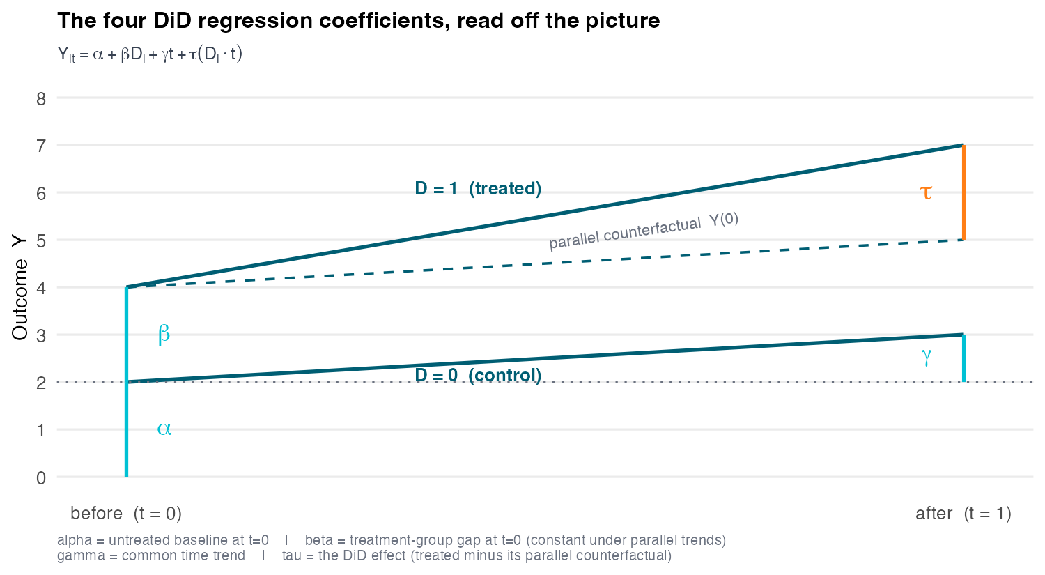
The fixed-effect form (Equation 15.3) is convenient on a panel, but it hides two coefficients worth seeing. Written out with the main effects visible, \[Y_{it} \;=\; \alpha \;+\; \beta\,D_i \;+\; \gamma\,t \;+\; \tau\,(D_i \times t) \;+\; \varepsilon_{it}, \tag{15.4}\] the DiD reads off four coefficients (Figure 15.3): \(\alpha\) the untreated baseline at \(t{=}0\), \(\beta\) the treatment-group gap at \(t{=}0\) (which must stay constant for parallel trends to hold — that is \(\beta\)’s role), \(\gamma\) the common time trend, and \(\tau\) the interaction, the DiD effect itself. On a panel, the unit fixed effects absorb \(\alpha + \beta D_i\) and the period fixed effects absorb \(\gamma t\), collapsing Equation 15.4 back to Equation 15.3, whose lone slope is this same \(\tau\) once the main effects are swept into the fixed effects. The treatment indicator is \(D\) throughout — \(D_i\) for treated-group membership, \(D_{it} = D_i \times t\) for the treated-and-post cells — matching the \(D\) and effect-coefficient \(\tau\) of S06–S09.

The interaction form earns its keep on data the pure unit-FE model cannot handle: repeated cross-sections, where different units are sampled before and after — survey waves, different houses listed pre- and post-highway, a fresh customer sample each period. There is no panel to attach unit fixed effects to, but Equation 15.4 still identifies the DiD from the four group×period means.

Figure 15.3: The four DiD regression coefficients read off the picture: \(\alpha\) the untreated baseline, \(\beta\) the treatment-group gap at \(t{=}0\) (constant under parallel trends), \(\gamma\) the common time trend, and \(\tau\) the gap between the treated path and its parallel counterfactual — the DiD effect.

Two periods is not the limit — only one common launch date is. Nothing in the 2×2 requires exactly two periods. If every treated unit launches on the same date (common, or “block”, adoption), the panel can span as many periods as you like and static TWFE (Equation 15.3) is still an unbiased, clean DiD: with a single launch date the only comparisons TWFE ever forms are treated-vs-not-yet-treated and treated-vs-never-treated, so the forbidden comparison that ruins staggered TWFE (Section 15.3.3.1) cannot arise — extra periods simply buy precision. More periods also buy something new for free: replacing the single treatment dummy with one coefficient per period-since-launch recovers the dynamic treatment effect — an event study whose launch date is shared by all treated units, whose leads should sit near zero and whose lags trace the ramp-to-plateau. We write that regression down and reuse it as a pre-trend diagnostic in Section 15.3.5.1. Everything here rests on that single shared date: real rollouts stagger adoption across units, so the shared launch date \(g\) becomes unit-specific \(g_i\) — and that one change is what breaks naive TWFE (Section 15.3.3.1) and later contaminates this very event study. The estimator is introduced here and reused there; the culprit throughout is timing variation, not panel length.

15.3.2.7 Parallel trends: the identifying assumption

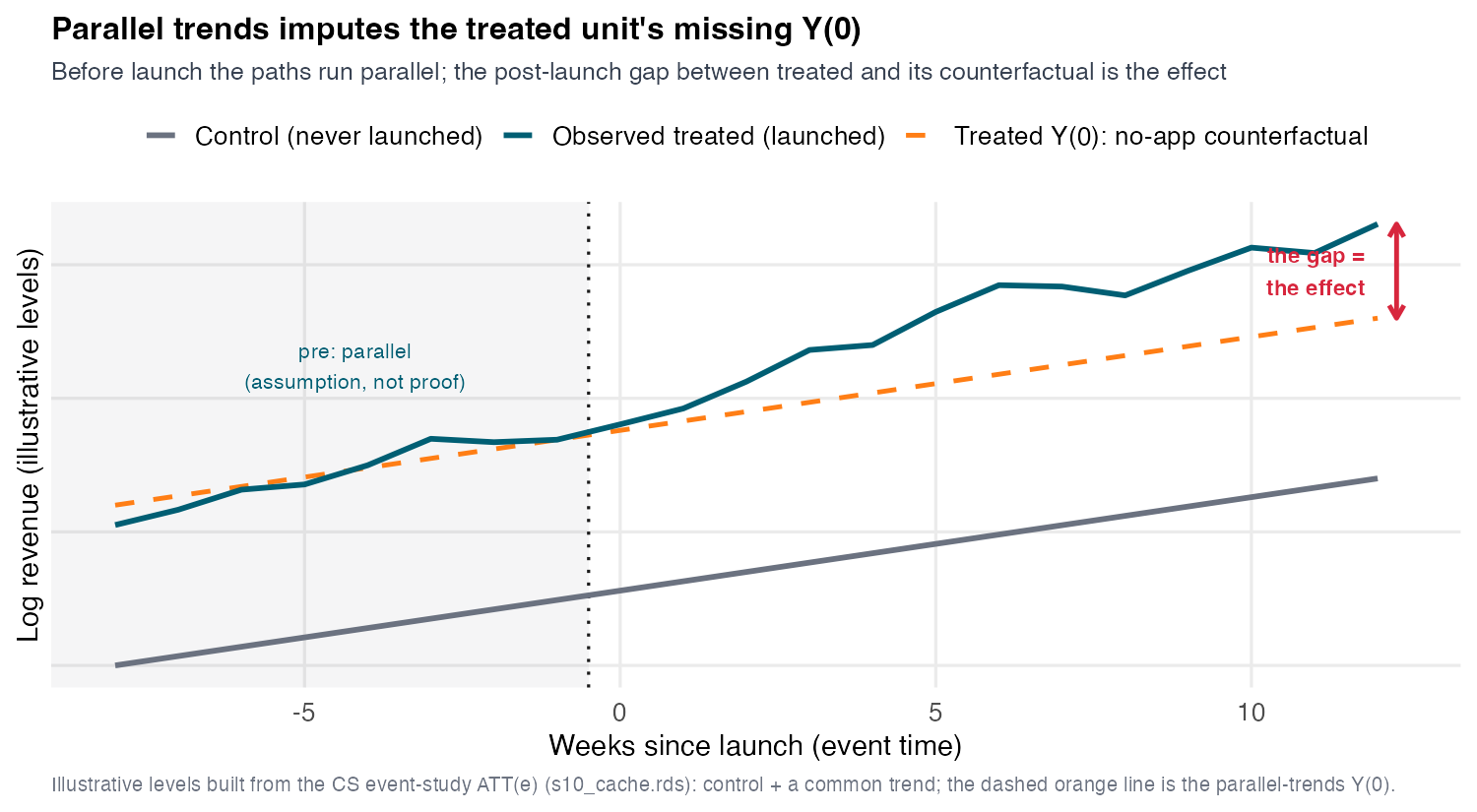
DiD identifies the ATT if and only if the treated units would have followed a path parallel to the controls had they not been treated — the dashed counterfactual \(Y(0)\) line in Figure 15.4. Formally, writing \(Y_{it}(0)\) for the never-treated potential outcome, parallel trends requires

\[\mathbb{E}\!\left[Y_{it}(0) - Y_{i,t-1}(0) \mid \text{treated}\right] \;=\; \mathbb{E}\!\left[Y_{it}(0) - Y_{i,t-1}(0) \mid \text{control}\right]. \tag{15.5}\]

Everything rides on this one claim, and it is fundamentally untestable: we never observe the treated market’s no-app path after launch, so we can never confirm Equation 15.5 directly. What the assumption does and does not require matters. It does not require equal levels (the lines can start far apart); it requires equal trends (the same slope absent treatment).

Figure 15.4: Parallel trends as imputation. Pre-launch, the treated and control markets move on parallel lines. At launch the treated path jumps above where it was heading; the dashed line continues parallel to the control, tracing the counterfactual \(Y(0)\). The post-launch vertical gap between the solid treated path and the dashed counterfactual is the treatment effect. DiD is valid iff that dashed line is the right counterfactual.

WarningLevels versus logs: parallel trends is not functional-form-free

Parallel trends is scale-dependent — trends that are parallel in levels are generally not parallel in logs, and vice versa, so the choice of outcome transformation is itself an identifying assumption, not a cosmetic one (Roth and Sant’Anna 2023). Roth and Sant’Anna show that parallel trends holds simultaneously under any strictly monotone transformation only in knife-edge cases (essentially, when treatment is “as good as random” or the counterfactual distribution is stable in a specific sense). The practical implication for BeanBuzz: we work in logs throughout — so effects read as percentages and the additive unit-plus-time model is multiplicative on the revenue scale — and we flag that this is a substantive modelling choice. If the true data-generating process had additive-in-levels seasonality, a log specification could manufacture or mask a violation. The discipline is to state the scale, justify it (here, revenue effects are naturally proportional), and check robustness to the alternative where it is cheap.

Parallel trends is the identifying assumption — a claim about the world — and it is worth separating cleanly from a second, purely mechanical problem. Even granting parallel trends, staggered treatment timing breaks naive TWFE estimation (Section 15.3.3.1): a different failure mode entirely, about how the clean 2×2s are combined, not about whether the comparison is valid. This session tackles the two in order. First, build a credible estimate (Section 15.3.3.1 through Section 15.3.3.14), granting parallel trends and fixing the estimation mechanics. Then interrogate the assumption itself (Section 15.3.5.1 through Section 15.3.5.4) — the event-study diagnostic and the HonestDiD sensitivity analysis. Estimate first, interrogate second; keep the two issues distinct.

15.3.2.8 The full ledger — three identifying assumptions, and the proof

Parallel trends does the visible work, but two more assumptions are doing quiet work and deserve names, so a reader can list the assumptions DiD requires — not just the famous one.

• (A1) Parallel trends (Equation 15.5) — the one you must defend with evidence.
• (A2) No anticipation — \(Y_{i,\text{pre}}(1) = Y_{i,\text{pre}}(0)\) for the treated: no effect before launch. This is what licenses a not-yet-treated market as a clean control (the Callaway-Sant’Anna move, Section 15.3.3.8), and it is probed jointly with parallel trends by the event-study leads (Section 15.3.5.1) — flat leads are evidence for parallel trends and no-anticipation, not parallel trends alone.
• (A3) SUTVA / no interference — one market’s launch does not move another’s revenue. In a geographic rollout this is a genuine, live threat (cross-market cannibalization or brand spillover across neighbouring markets), so it is argued, not assumed away; here the markets are treated as non-interfering.
• (A.pos) Positivity / overlap — binds only once you condition on covariates (Section 15.3.4.1); with no covariates it is automatic. Flagged here because on BeanBuzz it is exactly the assumption that breaks when you condition on market size.

Given consistency, parallel trends, and no anticipation, the double difference identifies the ATT, and the derivation is short enough to see. Start from the estimand (Equation 15.2); use no-anticipation (A2) to add and subtract the treated group’s pre-period, then parallel trends (A1) to swap the treated group’s unseen \(Y(0)\) change for the control’s observed one: \[ \begin{aligned} \tau_{\text{ATT}} &= \mathbb{E}[Y_1(1) - Y_1(0)\mid D{=}1] \\ &\overset{(A2)}{=} \big(\mathbb{E}[Y_1\mid D{=}1] - \mathbb{E}[Y_0\mid D{=}1]\big) - \mathbb{E}[Y_1(0)-Y_0(0)\mid D{=}1] \\ &\overset{(A1)}{=} \big(\mathbb{E}[Y_1\mid D{=}1] - \mathbb{E}[Y_0\mid D{=}1]\big) - \big(\mathbb{E}[Y_1\mid D{=}0] - \mathbb{E}[Y_0\mid D{=}0]\big). \end{aligned} \tag{15.6}\] Consistency turns each potential outcome into an observed mean, so the estimand equals the sample double difference — the +5.2% of Equation 15.1 is this identity evaluated on four cell means, not an analogy.

15.3.3 Act 3 — Staggered adoption

15.3.3.1 Why TWFE breaks under staggering

15.3.3.2 Real rollouts are a staircase

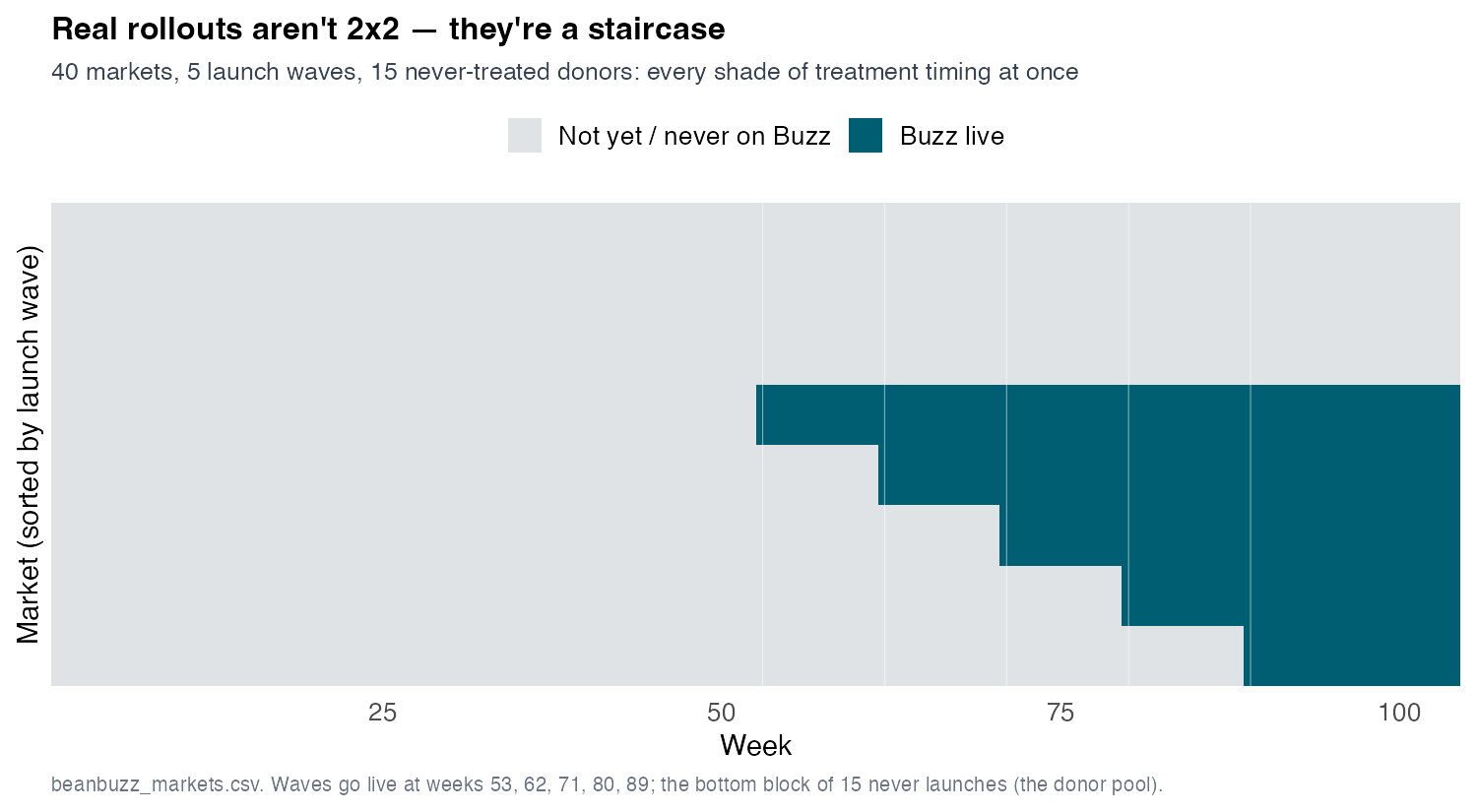
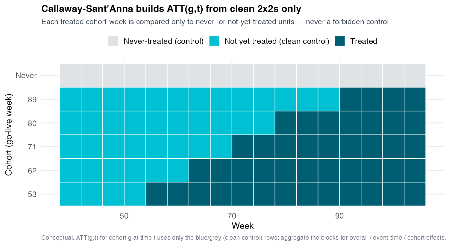
BeanBuzz is a panel of 233 stores in 40 markets over 104 weeks. The app launches in five staggered waves — weeks 53, 62, 71, 80, 89 — and 15 markets never get it, serving as clean donor controls throughout (Figure 15.5). At any given week some cohorts are already treated, some are about to be, some never will be. This staggered structure is what breaks the tidy 2×2 — and, as we will see, what breaks naive TWFE.

Figure 15.5: The adoption staircase (BeanBuzz): markets on the vertical axis, weeks on the horizontal. Five treatment cohorts switch on at weeks 53, 62, 71, 80 and 89, forming a descending staircase of treated cells, while 15 never-treated donor markets remain untreated across all 104 weeks. The 15 never-treated markets are uncontaminated controls available at every point in time; the robust estimators lean on them heavily.

15.3.3.3 The instinct, and the plausible-looking number it gives

The natural move is the same TWFE specification (Equation 15.3) that recovered the 2×2, now on the full staggered panel:

feols(log_rev ~ app_live | sid + week, data = panel, cluster = ~mid)

It runs and returns one tidy number: static TWFE = +3.7%, far below the naive +16.3%, so it looks like a responsible, confound-corrected estimate, and most practitioners would stop here. The trap is that +3.7% is biased — and biased in a subtle, non-obvious direction: dragged downward, below the true +4.9%, by comparisons the model should never have made. The bias is not omitted confounding (the fixed effects handle that); it is in the mechanics of how TWFE combines the staggered 2×2s when treatment effects grow over time.

15.3.3.4 The dynamic counterpart — the effect path

Static TWFE compresses everything into a single number; swap the single treatment dummy for a full set of event-time indicators and the same machinery returns the whole effect path — the dynamic TWFE event study, feols(log_rev ~ i(rel_time, ref = -1) | sid + week), one coefficient \(\beta_k\) per week \(k = t - g_i\) relative to each unit’s own launch \(g_i\). On BeanBuzz the leads hug zero and the lags ramp to a +3.2% plateau by event-week 8–12 (Figure 15.6) — the dynamics the single static coefficient hid. But it is the same naive estimator: under staggering its lags inherit the identical forbidden-comparison contamination — here mild, visible as the slight drift above the plateau at the far horizon. So we do not lean on the naive lags; the robust menu returns the trustworthy dynamic path (Section 15.3.3.8), and we re-read these leads as the pre-trend diagnostic in Section 15.3.5.1.

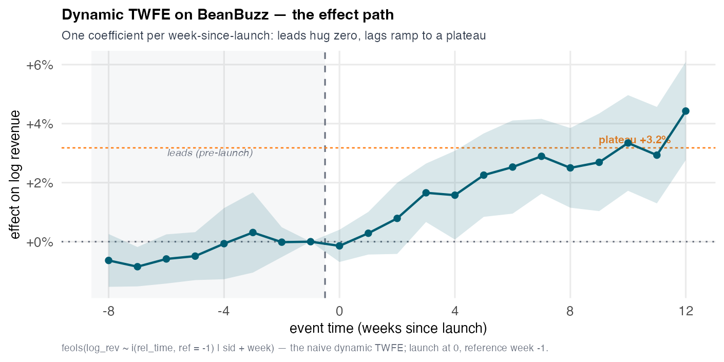
Figure 15.6: Naive dynamic TWFE on BeanBuzz (feols(log_rev ~ i(rel_time, ref = -1) | sid + week)): one coefficient per week-since-launch. Pre-launch leads hug zero; post-launch lags ramp to a ~+3.2% plateau (event-weeks 8–12). The far-horizon coefficient drifts slightly above the plateau — the mild forbidden-comparison contamination the robust estimators (Section 15.3.3.8) remove; the leads are re-read as a pre-trend diagnostic in Section 15.3.5.1.

15.3.3.5 TWFE secretly averages every 2×2 it can build

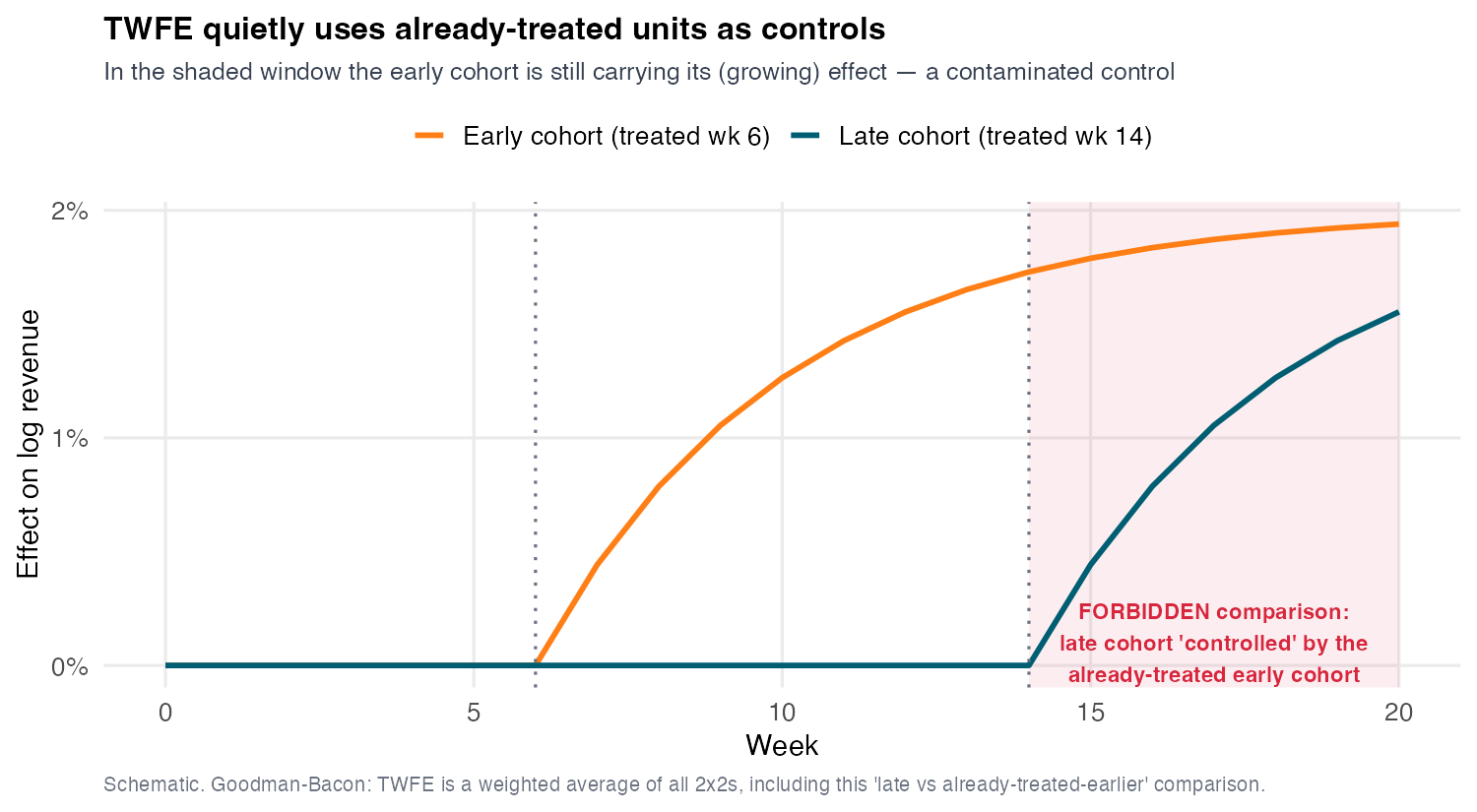
Goodman-Bacon’s decomposition is the analytical heart of the bias (Goodman-Bacon 2021): static TWFE on a staggered panel is a variance-weighted average of every 2×2 DiD in the data. Two of the three flavors are legitimate — treated vs never-treated (clean) and treated vs not-yet-treated (also clean, because a unit that will be treated later is a valid control while it is still untreated). The problem is the third flavor TWFE must form to exploit all the timing variation: using already-treated units as controls for later-treated units (Figure 15.7). That already-treated cohort is still responding to its own launch; if the effect grows over time, the control’s outcome is rising for treatment reasons, not just time. Subtracting that rising path over-subtracts, and the later cohort’s estimated effect is pulled toward zero. This is the forbidden comparison — “running the clock backwards.”

Figure 15.7: The forbidden comparison: a later-treated cohort differenced against an earlier-treated cohort that is already receiving the app. The earlier cohort’s own treatment effect is still evolving, so its change is not pure time — subtracting it contaminates the estimate. When effects grow over time, the contamination pulls the later cohort’s effect toward zero.

15.3.3.6 Where the weight goes — and the negative-weight algebra

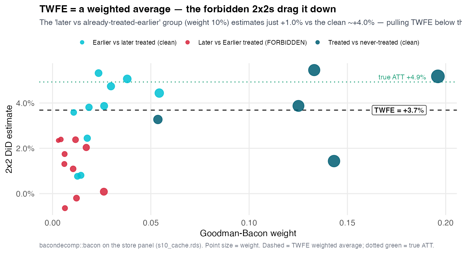
Plot each 2×2’s estimate against its Goodman-Bacon weight (Figure 15.8). The clean comparisons cluster near +4.0%; the forbidden “already-treated-as-control” group sits much lower, around +1.0%, yet still carries about 10% of the total weight. So TWFE’s +3.7% is a weighted blend that drags the honest ~+4% down toward the contaminated +1% — the forbidden group is a low-estimate anchor.

Figure 15.8: Every 2×2 in the BeanBuzz panel: horizontal position is its Goodman-Bacon weight, vertical position is its estimate. Clean treated-vs-never and treated-vs-not-yet comparisons cluster around +4.0%; the forbidden already-treated-as-control group sits near +1.0% while still carrying ~10% of the weight. The weighted average lands at +3.7%, dragged down from the clean ~+4% by the low-estimate forbidden cluster.

State the general pathology precisely so students do not overgeneralize. Writing static TWFE’s estimand as a weighted sum over the \(K\) underlying 2×2 comparisons,

\[\hat\tau^{\text{TWFE}} \;=\; \sum_{k} w_k\,\widehat{\text{DiD}}_k, \qquad \sum_k w_k = 1, \tag{15.7}\]

the de Chaisemartin–D’Haultfœuille decomposition shows that some weights \(w_k\) on the forbidden comparisons can be negative (Chaisemartin and D’Haultfœuille 2020). A weighted average where some weights are negative is not a treatment effect anyone asked for — in extreme cases TWFE can return the wrong sign, even when every underlying cohort effect is positive. Calibrate the BeanBuzz-specific claim carefully: here the forbidden group is attenuated (its estimate is +1.0% versus the clean +4.0%) and that low value drags the average down to +3.7%, biased toward zero from the true +4.9% — a contaminated, attenuated estimate, not literally a sign-flipping negative weight in this dataset. The deck’s honest framing: “biased toward zero / dragged down here; negative weights are the general worst case.”

15.3.3.7 The fix is a design principle, not a better regression

You cannot patch TWFE by adding controls or interactions — the problem is which comparisons it forms, not which variables it omits. The fix is a one-liner worth memorizing: never use an already-treated unit as a control; only compare treated cohorts to not-yet-treated or never-treated units. Every robust estimator in Section 15.3.3.8 and Section 15.3.3.14 is a disciplined way of enforcing that rule. Baker et al. (2025) frame this as forward-engineering — decide the estimand and the clean comparisons first, then derive the estimator — rather than running a regression and reverse-engineering what assumptions would make it valid.

15.3.3.8 Callaway-Sant’Anna ATT(g,t): the robust spine

15.3.3.9 One clean building block at a time

Callaway-Sant’Anna’s move is disaggregation: don’t force one pooled coefficient (the TWFE mistake) — estimate a separate, clean treatment effect for each cohort \(g\) and each period \(t\), the group-time ATT (Callaway and Sant’Anna 2021):

\[\text{ATT}(g, t) \;=\; \mathbb{E}\big[\,Y_t(g) - Y_t(0) \,\big|\, G = g\,\big], \tag{15.8}\]

where \(g\) is the cohort’s launch week (53, 62, 71, 80, 89) and \(t\) is the calendar period the effect is measured in. Each ATT\((g,t)\) is a transparent 2×2: cohort \(g\) compared only against units not yet treated at \(t\) (or never treated), with already-treated cohorts greyed out as ineligible controls (Figure 15.9). By construction the forbidden comparison is structurally impossible.

Figure 15.9: The Callaway-Sant’Anna estimator. Top: a single ATT(g,t) — the cohort launched at week \(g\) is compared only against never-treated and not-yet-treated markets, with already-treated cohorts greyed out as ineligible. Bottom: the clean building blocks aggregated into an overall summary and an event-time summary. Identification happens once, at the building-block level; aggregation is then a reporting choice.

15.3.3.10 The shared grid every robust estimator reads

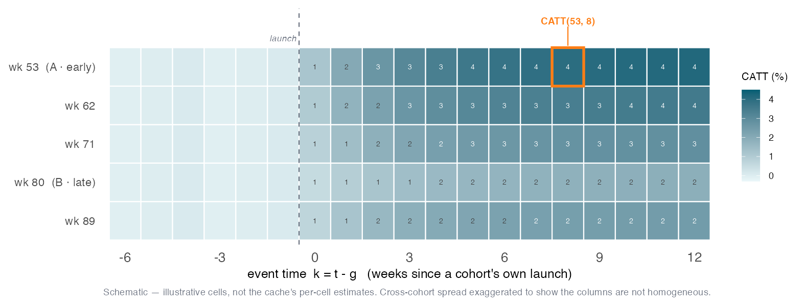
Line every cohort up by weeks since its own launch, \(k = t - g\), and one cell of the resulting grid is the cohort average treatment effect on the treated — the object every method in this act is really after:

\[\text{CATT}(g,k) \;=\; \mathbb{E}\big[\,Y_{g+k}(g) - Y_{g+k}(\infty) \,\big|\, G = g\,\big], \tag{15.9}\]

cohort \(g\)’s average effect \(k\) weeks after its own launch, measured against the never-treated baseline \(Y(\infty)\). Set \(t = g+k\) and this is exactly Callaway-Sant’Anna’s \(\text{ATT}(g,t)\) (Equation 15.8) read in event time — the same estimand, just re-indexed. The grid (Figure 15.10) is the definition: rows are the five launch waves, columns are event time \(k\), each cell one \(\text{CATT}(g,k)\). Read down a column and the cells are visibly not homogeneous — the wk-53 wave matures near +4%, the wk-80 wave near +2% — so the plateau height varies by cohort. That cross-cohort heterogeneity is what the naive event study will crush (Section 15.3.3.14); every robust estimator is a disciplined way of keeping the cells clean before pooling them. Sun-Abraham and CS target the identical cell but reach it with different clean controls and fits (non-nested parallel-trends assumptions), so the estimated cells need not coincide to the digit — which is why SA’s +3.5% and CS’s +3.3% differ by construction, not by noise.

Figure 15.10: The CATT(g,k) grid (schematic): rows are BeanBuzz’s five launch waves ordered earliest on top, columns are event time \(k\) from before to after launch. Pre-launch cells are pale (near zero); post-launch cells warm and ramp to a plateau whose height differs by cohort — the wk-53 wave settles higher than the wk-80 wave — so the columns are visibly heterogeneous. One cell (cohort A at \(k=8\)) is outlined as \(\text{CATT}(53,8)\). Illustrative cells.

15.3.3.11 Aggregate the blocks the way your question demands

The ATT\((g,t)\)s are raw material; how you average them answers different questions, with no new assumptions per report:

• Overall ATT — average across all treated cohort-periods: the headline “what is the app worth?” number. Two flavours: type = "group" size-weights the per-cohort effects (+3.3%, the number Callaway-Sant’Anna recommend and we carry forward), while the cruder type = "simple" cell-averages and over-weights the earlier, bigger cohorts (+3.5%).
• Event-study (dynamic) — average by time-since-launch: recovers the dynamic ramp-to-plateau (Figure 15.13). Its own single-number roll-up (+2.25%) sits below the plateau because it averages in the small early lags — a ramp-average, not a rival estimate of the mature effect.
• By calendar time — average by period: is the lift bigger some weeks than others (+3.2% overall)?
• By cohort — average by launch wave: do later waves respond differently? This is the panel GATE (below).

Cohort ATT(g)s are the GATE/RATE discipline in panels. In S09 the rule was: never trust an average effect until you have checked whether it hides real heterogeneity, using the GATE (group effects) and RATE (is targeting worth it?). The Callaway-Sant’Anna cohort aggregation is the panel analog — the ATT by launch wave is a GATE over cohorts, answering “do early and late waves respond differently?” If the cohort-specific effects scatter widely, the headline overall ATT is averaging genuinely different objects — the same apples-and-oranges warning S09 issued. So the building-block design is not just a bias fix; it is a heterogeneity diagnostic that lets you look inside the average before reporting it. The panel slogan mirrors S09’s: disaggregate before you aggregate, and do not trust an average until you have inspected its components. This is why CS hands you the ATT(g,t)s, not just one number.

On BeanBuzz the Callaway-Sant’Anna overall ATT (group-weighted aggregation, never-treated controls, doubly-robust estimation, SEs clustered on market) is +3.3% — the spine estimate, built entirely from clean 2×2s (Figure 16.15). This is the credible number in the sense that it is free of the TWFE pathology. It does not equal the true +4.9%; it sits a bit below, and that residual gap is deliberate and meaningful (Section 15.3.3.14). Do not say the estimator “recovers the truth” — say it lands in a tight, defensible band free of the forbidden-comparison bias.

Figure 15.11: Estimator forest (BeanBuzz), confidence intervals against the true ATT line at +4.9%. Naive pre/post at +16.3% sits far to the right (time-driven artifact); static TWFE at +3.7% below true (dragged down by forbidden comparisons); the robust cluster — Callaway-Sant’Anna +3.3%, Sun-Abraham +3.5%, Borusyak +4.2%, Gardner +4.2% — clusters at +3.3–4.2%, just below the true line. Convergence across independent methods is the credibility check; the residual gap to +4.9% is the omitted-factor clue.

15.3.3.12 The doubly-robust moment is AIPW-on-differences (the S09 callback)

Each ATT\((g,t)\) is estimated with a doubly-robust moment that is consistent if either the outcome (trend) model or the propensity (who-launches-when) model is correct. This is exactly the S09 AIPW score — now computed on first-differenced outcomes. Let \(\Delta Y_{it} = Y_{it} - Y_{i,g-1}\) be the change from the base period \(g-1\) to period \(t\). Differencing removes the unit fixed effect; the Sant’Anna-Zhao DR-DiD estimator is then the AIPW moment applied to \(\Delta Y\) (Sant’Anna and Zhao 2020):

\[\widehat{\text{ATT}}(g,t) \;=\; \mathbb{E}\!\left[\,\underbrace{\big(\hat m^{\,\text{tr}}_{g,t}(X) - \hat m^{\,\text{co}}_{g,t}(X)\big)}_{\text{outcome regression on } \Delta Y} \;+\; \underbrace{\frac{\hat w(X)}{\mathbb{E}[\hat w(X)]}\,\big(\Delta Y - \hat m^{\,\text{co}}_{g,t}(X)\big)}_{\text{propensity-weighted residual}}\,\right]. \tag{15.10}\]

This is the S09 machinery verbatim — the per-unit orthogonal score whose conditional expectation is the conditional effect — applied after we difference out the unit fixed effect. DR-DiD = AIPW-on-differences. Students do not need a brand-new estimator for panels: they already know the score; it just operates on differences now. Two properties carry over verbatim from S09. Double robustness: because the ATT(g,t) is built from the AIPW moment, it is consistent if either the trend/outcome model (how \(Y(0)\) would have evolved) or the propensity model (who launches when) is correctly specified — two chances to be right, a safety margin naive TWFE never has (Sant’Anna and Zhao 2020). Neyman orthogonality: the score’s insensitivity to first-order nuisance error lets you fit those nuisances with flexible machine learning without contaminating the ATT to first order — the panel face of Part IV’s CausalML machinery, elaborated where covariates enter the estimators (Section 15.3.4.1).

15.3.3.13 Two languages, one digit

The robust estimate is a property of the design, not the ecosystem. The same Callaway-Sant’Anna estimand, computed in R via did (att_gt to build the ATT(g,t)s, aggte to aggregate) and in Python via the differences package’s ATTgt, returns +3.3% in both — exact parity to the displayed digit. When two independent implementations of the same well-specified estimand agree exactly, it confirms the number is a property of the research design (clean comparisons, the chosen aggregation), not an artifact of a package’s defaults. The lab has students reproduce both.

15.3.3.14 Same target, different plumbing

Callaway-Sant’Anna is the spine, but it is not alone. Three more estimators target the same heterogeneity-robust ATT by different machinery — and none forms a forbidden comparison. Convergence across independent failure modes is the credibility argument.

• Sun-Abraham (Sun and Abraham 2021): saturate the event-study regression with cohort-by-event-time interactions and average only the interaction-weighted clean terms, sidestepping the contamination. BeanBuzz: +3.5%.
• Borusyak-Jaravel-Spiess (BJS) imputation (Borusyak, Jaravel, and Spiess 2024): the most transparent expression of the Part V spine — see the recipe below. BeanBuzz: +4.2%.
• Gardner two-stage (Gardner 2022): residualize the outcome on fixed effects estimated from untreated observations only, then regress the residual on treatment. BeanBuzz: +4.2%.

15.3.3.15 Sun-Abraham: cells, not columns

Sun-Abraham deserves a closer look because it fixes the naive event study in place, using the very same feols engine. The naive dynamic TWFE forces one coefficient per event-time column, pooling every cohort — so \(\beta_k\) picks up not only the column-\(k\) effect you wanted but a leak from every other column, because collapsing one column inside two-way fixed effects nets cohorts sitting at different maturities against each other (Figure 15.10). The leak’s cause is cross-cohort heterogeneity in \(\text{CATT}(g,k)\) (Equation 15.9) — if the dynamic path were identical across cohorts the leak would cancel — and its vehicle sets weights that can go negative, so a naive lag (and even a naive lead) can flip sign. This is a distinct pathology from Goodman-Bacon’s static forbidden-2×2 story (it is Sun-Abraham’s Proposition 2), and it is why a flat naive pre-trend plot is not a clean pre-trends test — a point that returns in Section 15.3.5.1. Sun-Abraham’s fix is to saturate the grid: replace the pooled column dummies with a full cohort × event-time interaction and hold the control cohorts (never-/last-treated) out of the interaction, so each coefficient \(\hat\delta_{g,k}\) is one clean \(\widehat{\text{CATT}}(g,k)\) cell — never a cross-cohort blend. Pooling the clean cells back is then a reporting choice with non-negative cohort-share weights replacing OLS’s implicit possibly-negative ones — the same disaggregate-first, aggregate-later spine as Callaway-Sant’Anna. Two honesty notes on the SA numbers: the event-study path \(\nu_k = \sum_g \text{share}_{g,k}\,\widehat{\text{CATT}}(g,k)\) ramps to the ~+3% plateau, but the overall +3.5% (summary(sa, agg="att")) is a whole-grid interaction-weighted cell average, not the horizon-average \(\tfrac{1}{|K|}\sum_k \nu_k\) (that ramp-average is what gives the dynamic-overall its lower +2.25%); and SA weights by cohort share while the CS headline weights by cohort size, so the SA +3.5% \(\approx\) CS-simple +3.5% is a dataset coincidence, not an identity — CS’s carried headline stays +3.3%.

15.3.3.16 The Borusyak imputation recipe literally fills the blank

BJS imputation is the cleanest bridge to S12, so slow down on it:

1. Using only untreated cells (never-treated markets plus every market’s pre-launch periods), fit unit + time fixed effects.
2. Impute each treated cell’s \(\hat Y_{it}(0)\) — the missing no-app value.
3. Average the gaps \(Y_{it} - \hat Y_{it}(0)\) over treated cells → the ATT.

\[\widehat{\text{ATT}}^{\text{BJS}} \;=\; \frac{1}{|\mathcal{T}|}\sum_{(i,t)\,\in\,\mathcal{T}} \big(Y_{it} - \hat Y_{it}(0)\big), \qquad \hat Y_{it}(0) = \hat\alpha_i + \hat\lambda_t, \tag{15.11}\]

where \(\mathcal{T}\) is the set of treated cells. This is literally filling the blanked-out \(Y(0)\) rectangle from the cold open, and it fills it with an additive unit-plus-time model — exactly parallel trends in imputation form. The house mnemonic is “fit white, predict grey”: fit the fixed-effect model on the white (untreated) cells, then predict \(\hat Y(0)\) onto the grey (treated) cells. Name the price, too: because every treated cell is anchored on that one model, BJS assumes parallel trends across all groups and all periods — the strongest PT claim on the menu, stronger than Callaway-Sant’Anna, which only needs PT against a chosen comparison group. That is the honesty tax for the cleanest bridge to S12. BeanBuzz BJS gives +4.2%.

NoteForward to S12

S12’s counterfactual-imputation methods (gsynth, matrix completion) re-read this exact recipe and swap the additive model \(\hat\alpha_i + \hat\lambda_t\) for a flexible interactive-fixed-effects / factor model that lets unit and time interact — relaxing parallel trends. So BJS is not just another estimator; it is the conceptual hinge to the last session of the course.

15.3.3.17 The robust family lands just below the truth

The robust cluster spans +3.3% to +4.2%; the true ATT is +4.9%. The estimators did not recover the truth — they sit systematically below it, and that residual gap is not noise, it is a clue. Its source in the simulated DGP is an omitted regional-economy factor — a slow, latent wave that whole regions ride together, and that treated and control markets load on by different amounts — a subtle parallel-trends violation too small for even a careful pre-trend test to catch (as the diagnostic in Section 15.3.5.1 will show). DiD assumes additive unit-plus-time effects and therefore cannot represent a factor that interacts unit and time, so it leaves this bias on the table. This is precisely the motivation for the rest of Part V: synthetic control (S11) matches on pre-treatment trajectories and can absorb such a factor; counterfactual imputation (S12) models it explicitly. The gap is the course’s argument for why DiD is the beginning, not the end. Resist any “our method recovers the truth” cliché — the honest summary is a tight, defensible band near +3–4%, free of the forbidden-comparison bias, sitting just below the truth.

15.3.3.18 Four routes, one estimand — how they relate and differ

Step back and the four robust estimators fall into two families by how each builds its clean counterfactual: aggregate clean 2×2s (Callaway-Sant’Anna’s ATT(g,t) blocks, Sun-Abraham’s CATT(g,k) cells) versus impute \(Y(0)\) (BJS and Gardner’s per-cell gaps). They differ on their clean-control set (CS uses not-yet + never; SA uses never / last-treated; the imputers use all untreated cells) and on their inference (uniform bands, cluster-robust, influence-function, two-stage). The load-bearing axis is parallel-trends strength, and it is a two-tier split, not a strict ladder: {CS, SA} sit together at the weakest tier — each needs PT only against its chosen clean control — while {BJS, Gardner} make the strongest claim, PT across all groups and all periods (every untreated cell must be a valid \(Y(0)\) anchor). Do not rank Sun-Abraham above Callaway-Sant’Anna: on this menu they make essentially the same clean-2×2 PT assumption. That is why convergence to +3.3–4.2% certifies the staggered-timing fix — none is idiosyncratically broken by the timing problem — but not identification: because all four share the additive-PT backbone, they miss the truth together, which is exactly what the next act (covariates) and then S11/S12 chase.

15.3.4 Act 4 — Conditioning on covariates

15.3.4.1 Conditioning on covariates — and why it doesn’t rescue BeanBuzz

Raw parallel trends can fail while a conditional version holds — treated and control move in parallel only within strata of covariates \(\mathbf{X}\): \[\mathbb{E}[\Delta Y(0)\mid D{=}1,\mathbf{X}] \;=\; \mathbb{E}[\Delta Y(0)\mid D{=}0,\mathbf{X}], \qquad \mathbf{X}\ \text{not affected by treatment.} \tag{15.12}\] Conditioning switches on two assumptions raw DiD never needed. Conditionally-no-anticipation — no pre-launch effect within each \(\mathbf{X}\)-stratum — is the honest completion of the identification trio. And positivity / overlap — every treated covariate profile must have controls that share it, \(0 < \Pr(D{=}1\mid\mathbf{X}) < 1\) — which raw DiD gets automatically but conditioning can break. Watch the second one: on BeanBuzz it is exactly the assumption that shatters when you condition on market size.

15.3.4.2 Which covariates actually confound a trend?

Two axes decide whether a covariate can make conditional PT (Equation 15.12) bite: is the covariate itself fixed (\(X_i\)) or moving (\(X_{it}\)), and is its effect on \(Y\) time-invariant or time-varying?

• A fixed \(X_i\) with a fixed effect is a pure level gap — the unit fixed effect \(\alpha_i\) absorbs it, harmless.
• A fixed \(X_i\) with a time-varying effect confounds: different group levels times a changing loading produce a differential trend (urban markets swinging harder as seasonality peaks).
• A moving \(X_{it}\) confounds only if the groups’ covariate means evolve differently.

The fact that governs everything downstream: in any within/fixed-effect regression a strictly time-invariant regressor is collinear with \(\alpha_i\) and silently dropped. So a fixed \(X_i\) entered additively does nothing — it is exactly what plain DiD already differences out. It bites only through a time-varying channel: \(X_i \times t\) (in TWFE / Sun-Abraham / imputation) or CS’s differenced-outcome nuisances (differencing removes \(\alpha_i\), so the baseline \(X\) survives). The recurring test is therefore “does \(X\) move the trend, or just the level?” — only trend-movers qualify, which is why every per-estimator entry below uses \(X\times t\), not \(+X\).

Selection is not confounding. A covariate can also predict who gets treated (\(X\to D\)), but that alone does not bias DiD: differencing absorbs fixed levels, so DiD tolerates selection on time-invariant traits — it is built for it. Selection bites only if the selector also moves the trend. Two riders follow: do not reflexively condition on a pure selection driver (a strong one you don’t need can only hurt), and — the sharp irony — the stronger a covariate drives selection, the more conditioning on it breaks overlap, because a near-deterministic selector pins the propensity at 0/1.

15.3.4.3 Time-varying \(X\): pin it, or impute \(X(0)\)

Most estimators treat every covariate as time-invariant, fixing a moving \(X_{it}\) at its pre-launch value — both because a post-launch \(X_{it}\) the app itself changed is a mediator (a bad control, below) and because it cuts dimensionality. The cost is real: a covariate that genuinely evolves differently across groups is then left uncontrolled, and that particular PT violation survives. If \(X_{it}\) is exogenous to treatment given its past, the doubly-robust route may use its post-treatment values, or — the imputation family’s distinctive trick — you can impute the counterfactual \(X_{it}(0)\) on the untreated cells (the same fit-white / predict-grey recipe) and feed that into the \(Y(0)\) model (Caetano et al. 2024). On BeanBuzz all four adjustment covariates are strictly time-invariant, so this rung is the theory you’d need if they weren’t.

15.3.4.4 Which covariates? The bad-control trap

More covariates is not safer. A covariate the treatment affects — a mediator or any post-treatment variable — is a bad control: conditioning on it subtracts part of the effect (over-control), the same good-control / bad-control logic from S02 and S06 in a DiD setting (Caetano et al. 2024). The “kitchen-sink” TWFE that throws in every \(X_{it}\) can bias the estimate rather than clean it. The rule: condition only on pre-treatment characteristics that could confound the trend, never on a consequence of the app — exactly the call Assignment V’s Part B grades (the staffed_lanes bad control).

15.3.4.5 Where \(X\) enters each estimator

Each family takes covariates through a different door, and the door is the point:

• Covariate-TWFE and Sun-Abraham are one feols regression, so \(X\) enters as the same hand-written term — a fixed \(X_i\) with a time-varying effect as + i(week, X) (i.e. \(X_i \times t\)), a moving \(X_{it}\) with a constant effect as + X (Zeldow and Hatfield 2021). Only the treatment block beside it differs (i(rel, ref=-1) for TWFE, sunab(g, week) for Sun-Abraham). The price (Caetano-Callaway): the additive-linear form bakes in an effect homogeneous and linear in \(X\), adjusting changes not levels — and on TWFE the covariate merely decorates a still-biased estimator (covariates do not touch the staggered-timing bias), whereas on Sun-Abraham it rides an already-clean one.
• Callaway-Sant’Anna’s doubly-robust default puts \(X\) into two nuisance models on the change \(\Delta Y = Y_t - Y_{g-1}\) (differencing sweeps out \(\alpha_i\)): an outcome / trend model \(\hat m_0(\mathbf{X}) = \mathbb{E}[\Delta Y \mid D{=}0, \mathbf{X}]\), the control group’s expected change imputed onto the treated (Heckman, Ichimura, and Todd 1997), and a propensity model \(\hat e(\mathbf{X}) = \Pr(D{=}1\mid\mathbf{X})\) reweighting the controls to the treated’s \(\mathbf{X}\)-mix (Abadie 2005), combined in the AIPW-on-\(\Delta Y\) moment (Sant’Anna and Zhao 2020) — consistent if either is right (which is why did’s default is est_method = "dr"). Because that score is Neyman-orthogonal, both nuisances can be fit with flexible machine learning without first-order bias in the ATT — this is Chang’s double/debiased DiD (Chang 2020), the panel carry-over of Part IV’s CausalML that we flagged at Section 15.3.3.8; the reported BeanBuzz menu stays CS / SA / BJS / Gardner, so we add no separate DML number.
• BJS and Gardner put \(X\) in the \(Y(0)\) imputation — the untreated-cell first stage becomes \(Y_{it}(0) = \alpha_i + \gamma_t + \delta\,(X_i\times t)\), then predict onto the treated cells. Because there is no propensity model, there is no overlap requirement (an advantage on BeanBuzz), but they are outcome-model-only, so not doubly robust: a misspecified \(Y(0)\) model biases them with no backstop. BJS and Gardner take covariates identically and still coincide to the digit.

15.3.4.6 Seven candidates, one real confounder

BeanBuzz ships seven candidate covariates, and enumerating them is the exercise: a covariate confounds only if it moves the trend and lines up with the biggest-first rollout. The time-invariant ones — market_size, urban_share, seats, competitor_density — each carry a plausible “would confound if… → \(X_i\times t\)” story, but only urban_share actually does: it loads the winter-seasonality factor, so it is the genuine \(X\times t\) channel (drawn independently of size, so its bias is mild). market_size sets the revenue level (absorbed by \(\alpha_i\)) and drives the rollout — so its real damage is breaking overlap when you condition on it, not trend confounding. seats and competitor_density are decoys that never enter revenue. Among the time-varying ones, footfall_index and temp_c are proxies of the common seasonality (absorbed by \(\gamma_t\)), and mktg_spend jumps at launch — a treatment-affected bad control. So the honest roster reduces to adjust urban_share via \(X\times t\); do not over-condition on market_size; ignore the rest — plus a latent regional factor no observed \(X\) proxies.

15.3.4.7 The covariate forest: \(X\) rescues none of them

Condition each estimator its own way and the result is a deliberate non-result (Figure 15.12), computed on the student panel: static TWFE + urban_share × \(t\) lands at +3.5%, Sun-Abraham + \(X\) at +3.4%, Callaway-Sant’Anna doubly-robust with all four covariates at +3.9%, and BJS = Gardner + \(X\) at +4.2%. Two lessons. First, the covariate-adjusted band (+3.4–4.2%) is no tighter and no closer to the true +4.9% than the no-covariate robust menu (+3.3–4.2%) — covariates buy model-dependence, not accuracy. Second, and sharper: conditioning the CS-DR estimator on market_size — the biggest-first selection driver — pins the propensity at 0/1, throws 412 overlap-violation warnings, and blows its confidence interval wide open (roughly −3% to +11%). That is positivity failing in the code, not the textbook — the doubly-robust estimator you’d reach for is exactly the one overlap wrecks. And the deepest reason the covariates cannot rescue the estimate: the one covariate that genuinely moves the trend, urban_share, proxies the seasonality loading — the weak wave. The wave that actually does the damage is the latent regional-economy factor, and no observed covariate proxies it. Adjusting for urban_share therefore buys a real but nearly irrelevant correction: you are controlling for the wrong wave. Representing the right one needs the factor models of S11 (synthetic control) and S12 (counterfactual imputation), not more controls.

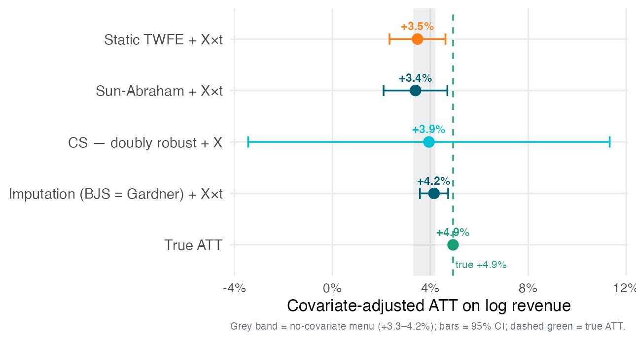
Figure 15.12: The covariate forest (BeanBuzz): four covariate-adjusted staggered-DiD estimators with 95% CIs against the true ATT at +4.9%. Static TWFE + urban_share × \(t\) at +3.5%, Sun-Abraham + \(X\) at +3.4%, Callaway-Sant’Anna doubly-robust with all four covariates at +3.9% with a very wide interval (~−3% to +11%) because conditioning on market_size breaks overlap, and the combined BJS = Gardner + \(X\) at +4.2%. All four sit inside the grey no-covariate band (+3.3–4.2%), all below the true +4.9% — covariate adjustment neither tightens the band nor reaches the truth.

15.3.5 Act 5 — Parallel trends

15.3.5.1 The event study as diagnostic — and its limits

Parallel trends is untestable, so we escalate. Our headline +3.29% (Callaway-Sant’Anna, group-weighted, Section 15.3.3.8) rests entirely on parallel trends (Equation 15.5) — a claim about the treated markets’ revenue had they never launched, a path that unfolds after launch and is never observed, so a flat pre-trend is circumstantial evidence, never proof. We climb three rungs of accelerating rigor: (i) eyeball the pre-trend — the visual test we are repairing, not one of the fixes → (ii) pretrends power, which quantifies how blind the eyeball is to a slow drift (Roth 2022) → (iii) HonestDiD, a continuous sensitivity analysis that subsumes the binary pre-test entirely (Rambachan and Roth 2023). Carry one honesty note through all three: the headline we quote to the CFO is the +3.29% cohort-size-weighted overall, whereas the sensitivity analysis of Section 15.3.5.4 brackets the +2.25% average post-launch effect — a different, more conservative aggregation of the same clean cells (it averages in the small early lags, so it sits below the +2.95% mature plateau). The +3.29% headline is not separately shielded; it leans on the very same parallel-trends assumption these tools stress-test.

In the pre-period both the treated and control paths are observed and not yet contaminated by treatment, so we can gather circumstantial evidence. The event study writes this as a regression: replace the single treatment dummy with one coefficient per event-time \(k = t - g_i\) (weeks since that unit’s launch), normalized at \(k=-1\):

\[Y_{it} \;=\; \alpha_i + \gamma_t + \sum_{k \neq -1} \beta_k \,\mathbb{1}[\,t - g_i = k\,] + \varepsilon_{it}. \tag{15.13}\]

Negative event times are leads (\(\beta_k, k<0\), pre-treatment), positive are lags (\(\beta_k, k>0\), post-treatment). In fixest this is the one-liner feols(log_rev ~ i(rel_time, ref = -1) | sid + week): i() expands rel_time into the indicator set, ref = -1 drops the normalization period, and the two fixed effects absorb \(\alpha_i, \gamma_t\). One caveat — a callback to Section 15.3.3.1: under staggered adoption this naive dynamic TWFE inherits the very same forbidden-comparison bias — its lag coefficients are weighted sums that borrow already-treated cohorts. So we do not read the naive lags; we read the robust event study: the Callaway-Sant’Anna dynamic aggregation (our spine, Section 15.3.3.8), or equivalently Sun-Abraham’s saturated version of this same regression, which drops the contaminated interaction terms. Figure 15.13 overlays all three — the naive TWFE, Sun-Abraham, and the Callaway-Sant’Anna aggregation; Lab 2 fits them.

Figure 15.13: Event study (BeanBuzz), three estimators overlaid on event time −8…+12 with market-clustered 95% CIs and a universal \(k=-1\) reference: naive dynamic TWFE (orange), Sun-Abraham (purple), Callaway-Sant’Anna (petrol). The leads hug zero — the largest pre-period coefficient is 0.74 pp and none is individually significant. Post-launch, Sun-Abraham and Callaway-Sant’Anna coincide on a matured plateau of +2.95% (Sun-Abraham is the regression-level de-contamination of the naive event study and on this data lands exactly on the CS aggregation, so the two plot as one line, annotated “SA = CS”), while only the naive TWFE drifts up to +4.43% by week 12 — the forbidden-comparison contamination the robust estimators remove, made visible.

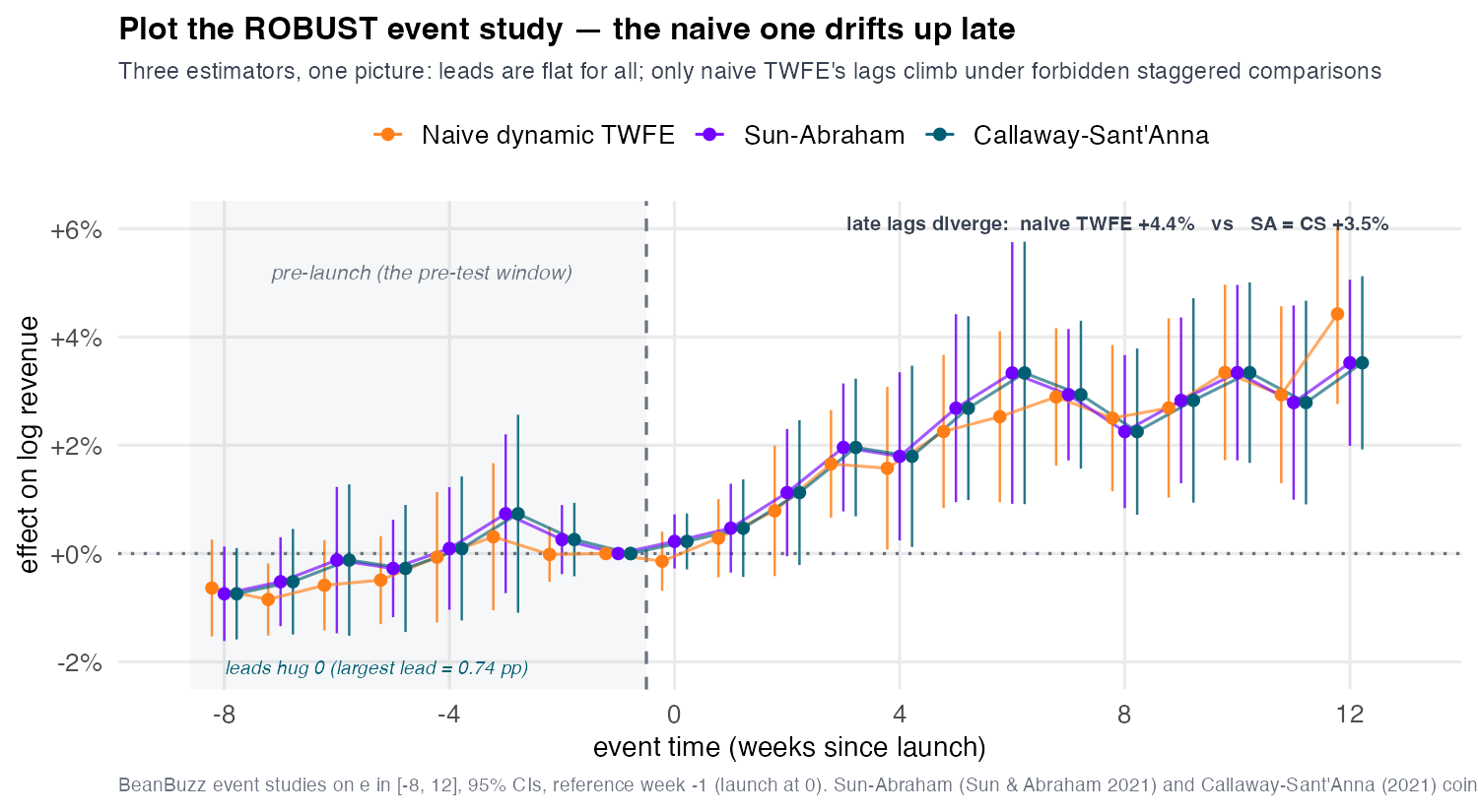
Read two things. The leads test the pre-period: if the treated and control trends were parallel before launch, the lead coefficients should hover around zero. On BeanBuzz the largest pre-period coefficient is just 0.74 pp in magnitude and none is individually significant — by eye the larger treated markets and the donor markets were moving in parallel before the app. The lags trace the dynamic treatment effect: the robust estimators (Sun-Abraham and Callaway-Sant’Anna, coincident here) ramp to a matured +2.95% plateau by event-week 8–12, consistent with an effect that builds as app adoption diffuses, while the naive dynamic TWFE drifts up to +4.43% by week 12 — the forbidden-comparison contamination the robust versions strip out. This is the strongest circumstantial evidence for parallel trends we can assemble, and a referee would expect to see exactly this plot.

The eyeball read of the leads has a formal counterpart, and naming it makes the “evidence, not proof” caveat precise. The pre-test is a joint hypothesis test that the pre-period lead coefficients are all zero — \(H_0:\beta_k = 0\) for every \(k<0\); “the pre-trend passes” means we fail to reject \(H_0\), which is not the same as accepting parallel trends. Whether that failure to reject is reassuring turns entirely on the test’s power: could it have detected a violation large enough to matter? This is exactly what Roth (2022)’s pretrends package quantifies — from the event study’s estimated covariance it computes the power of the pre-test against any hypothesized pre-trend and, inverting the question, returns the trend slope the test would catch with a target probability (slope_for_power(targetPower = 0.5) gives the slope caught half the time). Lab 3(c) runs exactly this on BeanBuzz; the slope it returns is the “low power” caveat below made concrete (Figure 15.14).

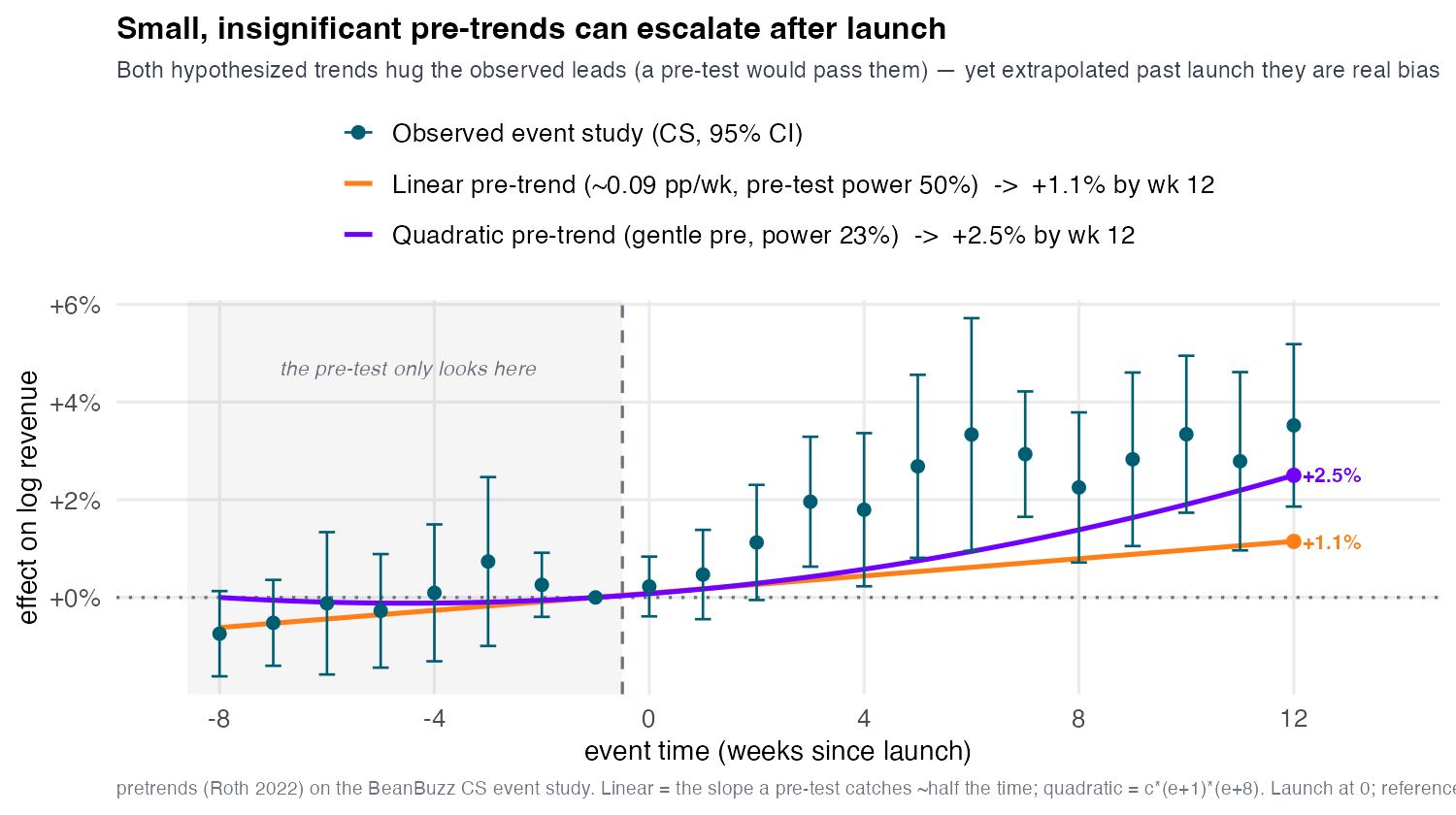
Figure 15.14: What a pre-test would miss on BeanBuzz (pretrends). Petrol: the observed Callaway-Sant’Anna event-study coefficients (95% CIs) — flat leads, lags climbing to ~+3.5% by week 12. Two hypothesized pre-trends are anchored at the \(k=-1\) reference and both sit inside the leads’ confidence intervals across the shaded pre-period — a pre-test would pass them — yet both grow into real post-launch bias. Orange: a linear drift of ~0.088 pp/week, caught only about 50% of the time, reaching +1.15% by week 12. Purple: a quadratic \(\delta(e)=c(e+1)(e+8)\) — shaped (its second root at the far lead) to stay even flatter in the pre-window — caught only ~23% of the time, yet curving up faster to +2.5% by week 12. The lesson: among violations a pre-test cannot distinguish from flat, a convex one does more post-period damage than a linear one, which is why we escalate from pre-testing to the sensitivity analysis of Section 15.3.5.4.

15.3.5.2 A flat pre-trend does NOT prove parallel trends

Say this slowly — it is the single most-violated principle in applied DiD. A flat, insignificant pre-trend is evidence, not proof, for three reasons:

• Low power. Pre-tests frequently fail to detect trend differences large enough to badly bias the estimate; a slow drift can hide inside wide confidence intervals. Absence of a significant pre-trend is not evidence of absence (Roth 2022).
• Wrong window. Parallelism over a handful of observed pre-weeks says nothing about whether a divergence opens up in the unobserved post-period.
• Conditioning bias. The common practice of keeping a study only if it “passes” the pre-test selects on noise and distorts the reported estimate.

NoteRoth (2024): the pre-test has a power cost, and event-study plots can mislead

Two further subtleties make the event study a sharper tool than the casual eyeball read. First, power: Roth (2022) quantifies how often a pre-test misses a trend difference large enough to overturn the conclusion — for BeanBuzz, the pretrends power analysis (Lab 3) shows a linear drift of about 0.09 pp/week would be caught only about half the time, so “flat over eight weeks” is fully consistent with a slow drift that compounds into real bias over the post-horizon. Second, construction artifacts: Roth (2024) shows that modern robust estimators build pre- and post-coefficients asymmetrically (CS uses short differences pre, long differences post; BJS compares to different reference periods), so a default event-study plot can display a kink or jump right at the treatment date even with no effect and no pre-trend. The practical rule: use a universal base period for CS event-study plots (the base_period = "universal" option, which is also what the HonestDiD helper requires), and treat the pre-period as a sensitivity yardstick (Section 15.3.5.4), not a pass/fail gate.

15.3.5.3 HonestDiD: the honest question

The constructive response to “flatness is not proof” is to stop treating the pre-test as a binary gate and start treating it as a yardstick. The honest question is quantitative: how large a post-launch parallel-trends violation — measured against the worst wobble we actually observed pre-period — would it take to overturn our conclusion? The answer is a single interpretable number, the breakdown value, due to Rambachan and Roth (2023). The object we stress-test is the +2.25% average post-launch effect (mean of the dynamic lags \(e=0\ldots12\) — the board-relevant object, exactly what Lab 3’s l_vec = rep(1/npost, npost) targets), not the +3.29% cohort-size-weighted headline; the very next section (Section 15.3.5.4) computes its breakdown. The reframe is the spine of this parallel-trends module — from “did the pre-trend pass?” to “how big a violation would overturn our number?”

15.3.5.4 HonestDiD mechanics: breakdown values

Now cash the check from Section 15.3.5.3. We have the +2.25% average post-launch effect — so we can stress-test it. Rambachan and Roth (2023) replace the binary pre-test with a continuous sensitivity analysis: instead of asking “did pre-trends pass?”, trace how the conclusion degrades as we admit larger parallel-trends violations, and report the violation size at which it flips.

15.3.5.5 Bound the post-period violation by the worst pre-period one

We never observe the post-launch violation, but we did observe the pre-launch deviations from parallelism, so we anchor to them. The relative-magnitudes restriction caps the post-period violation at a multiple \(\bar M\) of the largest pre-period violation:

\[\big|\,\delta_t^{\text{post}}\,\big| \;\le\; \bar M \cdot \max_{s\,<\,0}\big|\,\delta_s^{\text{pre}}\,\big| \qquad \text{for all post-periods } t, \tag{15.14}\]

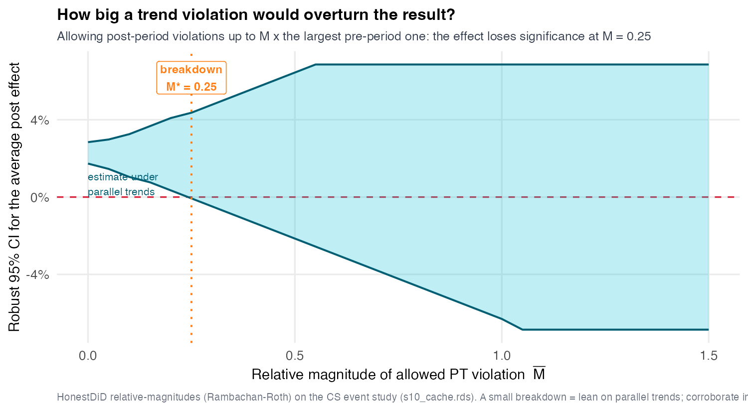
where \(\delta\) denotes the (unobserved post / observed pre) deviation from parallel trends. \(\bar M = 1\) says “assume the post-period trends could diverge as badly as the worst divergence we saw pre-period”; \(\bar M = 0.25\) says “a quarter as bad”; \(\bar M = 2\) says “twice as bad.” For each \(\bar M\), HonestDiD computes the identified set and a confidence interval for the +2.25% average post-launch effect (the mean of the dynamic lags \(e=0\ldots12\), Figure 15.15). At \(\bar M = 0\) (exact parallel trends) you recover a clearly-positive interval — the original-OLS interval is [+1.58%, +2.92%], and the conditional least-favorable (C-LF) sweep the figure plots starts a touch tighter at [+1.73%, +2.84%]; as \(\bar M\) grows the interval widens and its lower bound falls toward zero — the more you doubt parallel trends, the less you can conclude — reaching [−0.07%, +4.36%] at the breakdown \(\bar M^{*} \approx 0.25\).

Figure 15.15: HonestDiD sensitivity (BeanBuzz, relative-magnitudes), stress-testing the +2.25% average post-launch effect. Horizontal axis: \(\bar M\), the allowed post-period violation as a multiple of the largest pre-period violation. Vertical axis: the robust ATT confidence interval. At \(\bar M = 0\) the plotted C-LF sweep interval is [+1.73%, +2.84%] (the original-OLS parallel-trends interval is the slightly wider [+1.58%, +2.92%]), clearly above zero; as \(\bar M\) increases the interval widens and its lower bound falls, first crossing zero at the breakdown value \(\bar M^{*} \approx 0.25\), where it reaches [−0.07%, +4.36%].

15.3.5.6 The breakdown value

The breakdown value \(\bar M^{*}\) is the smallest violation (in units of the worst pre-period wobble) at which the confidence interval first includes zero — the smallest doubt about parallel trends sufficient to overturn the conclusion that the app helped. Large \(\bar M^{*}\) → hard to overturn → robust; small \(\bar M^{*}\) → a mild violation suffices → fragile. It collapses the whole sensitivity curve into one communicable number.

WarningBeanBuzz: statistically clear, only moderately robust

BeanBuzz’s breakdown value is \(\bar M^{*} \approx 0.25\). A post-launch parallel-trends violation only a quarter as large as the worst wobble we saw pre-period is enough to push the lower confidence bound to zero and overturn the average post effect. Why so small when the pre-trends looked flat? Because the bias on the average post effect compounds over the post horizon — a slow drift that is invisible week-to-week accumulates over the plateau period into something large enough to matter (and recall the pretrends analysis: a linear drift of ~0.09 pp/week would be caught only about half the time). So the correct reading is nuanced and must not be softened into a triumph: the effect is statistically clear under parallel trends but only moderately robust to violations of it — not bulletproof. Explicitly do not claim “the effect survives violations larger than anything we observed.” Be precise about scope, too: it is the +2.25% average post-launch effect that is moderately robust; the +3.29% cohort-weighted headline leans on the same parallel-trends assumption but is not separately shielded by this sensitivity analysis. The honest takeaways: report a band, not a point; flag that flat pre-trends over a few weeks cannot rule out a slow drift; and corroborate with a method that does not lean on parallel trends — synthetic control in S11.

15.3.5.7 Pointer: the ARP / FLCI machinery underneath

The mechanics above ride on Rambachan and Roth (2023)’s broader framework, which we use but do not derive in full. Two pieces are worth naming for students who go deeper. The confidence intervals are constructed by inverting moment-inequality tests — the Andrews-Roth-Pakes (ARP) conditional/hybrid tests — over the partially-identified set implied by Equation 15.14. When the violation is restricted to a smoothness class (bounded second differences) rather than relative magnitudes, the optimal interval is the fixed-length confidence interval (FLCI), which trades a small amount of coverage robustness for a much shorter band. The HonestDiD package implements both; the relative-magnitudes route we report is the most intuitive parameterization for a business audience because it is anchored to an observed quantity (the worst pre-period wobble). For the full ARP/FLCI theory — test statistics, the least-favorable and conditional critical values, and the smoothness-class derivations — see Rambachan and Roth (2023).

15.3.5.8 The Part V discipline, in one workflow

1. Identify — state the assumption (parallel trends) and the clean comparisons it licenses.
2. Impute — fill the missing \(Y(0)\) with the additive unit + time model (CS / BJS).
3. Report a band + breakdown — never a naked point. How wrong could we be, and how much would it take?

This is the same honesty discipline as S09’s “is it real?”, moved from heterogeneity to panels. A point estimate without a sensitivity analysis is not a finding.

15.3.5.9 Extensions you’ll meet in the lab

The clean-comparison recipe generalizes — each variation bends one part of it without re-teaching the whole. These are pointers, exercised in the take-home:

• Continuous / dose treatment. When treatment is an intensity (marketing spend, mktg_spend) rather than on/off, parallel trends must hold at every dose level, and the building-block estimators have dose-response analogs. Watch the assumption strengthen: “no differential trend” becomes “no differential trend at any dose.”
• Count outcomes. Revenue is continuous, but transaction counts (transactions) call for a Poisson / log-link DiD (fepois in R, pyfixest in Python). The additive unit-plus-time structure moves to the log scale; the no-forbidden-comparison logic is unchanged.
• Too few clusters. With only 15 donor markets (and ~25 treated clusters), standard cluster-robust standard errors over-reject — they find significance too easily. The fixes widen the interval honestly: CR3 (a bias-reduced cluster-robust variance, clubSandwich in R) and the wild-cluster bootstrap (wildboottest in Python). The lab shows naive SEs over-rejecting and the corrections restoring honest coverage.

NotePointer: hidden linearity in dose / continuous DiD (Caetano-Callaway)

A subtle trap specific to continuous treatment: even within the clean-comparison framework, a naive TWFE or two-way Mundlak specification on a continuous dose can impose a hidden linearity — it implicitly assumes the dose-response is linear and that there is no selection into dose level on the basis of trends. The group-time logic of Callaway and Sant’Anna (2021) must be extended to dose-time, and the comparison set must additionally rule out selection on the dose. Caetano and Callaway show that the standard continuous-DiD estimands recover a causal response only under a “no-selective-trends-by-dose” condition that is easy to violate and rarely stated. For BeanBuzz’s marketing-spend take-home, the practical takeaway is to treat the continuous-dose result as illustrative, not definitive, and to flag the extra assumption explicitly rather than letting the regression hide it.

15.4 Coding Lab

The lab works the BeanBuzz difference-in-differences problem end to end on a simulated panel where the truth is known (true ATT = +4.9%), so each exercise is a recovery check, not a graded discovery — Assignment V will use a different domain, so nothing here pre-solves it. The arc follows the headline: build the 2×2 by hand, see the TWFE bias and where Goodman-Bacon sends the weight, watch four robust estimators converge to one plateau, then ask honestly how wrong parallel trends could be — closing on the honest band-and-breakdown verdict and the extensions you’ll meet in the take-home. Each exercise gives a Scaffold with # ___ YOUR CODE placeholders in both R and Python; attempt it, then expand Show solution to compare. The solutions mirror the verified pipeline in materials/data/make_s10_cache.{R,py} and reproduce the locked numbers.

Download the data: beanbuzz_panel.csv (the store-week staggered panel — 233 stores × 104 weeks) and beanbuzz_markets.csv (the market-week aggregate used for Lab 0’s by-hand 2×2).

WarningHonest R ↔︎ Python parity caveat

The two languages share the clean, both-stack steps and diverge only where the ecosystems do. Callaway-Sant’Anna ATT(g,t) is exact-parity: R did::att_gt + aggte and Python differences.ATTgt both land on +3.3% (group-weighted, never-treated controls, doubly-robust). Four asymmetries are stated plainly rather than papered over:

• Goodman-Bacon (Lab 1) has no clean Python implementation, so it is R-only; Python students read the pre-baked R output (the forbidden group’s weight and estimate) and one sentence of interpretation.
• HonestDiD and pretrends (Lab 3) are R-only; Python students read the pre-baked R sensitivity table and the honest takeaway.
• The CR3 few-cluster correction (take-home) is R-led; Python’s wildboottest covers the few-cluster point.

Beyond CS, the robust menu is R-led: Sun-Abraham (fixest::sunab), BJS (didimputation), and Gardner (did2s) are shown R-side, with the Python event study via pyfixest and the CS aggregations via differences.

Notation: the store panel derives first_treat from go_live_week (an Inf go-live → 0, the never-treated code), uses numeric store/market ids, and clusters SEs on market (the ~25 treated clusters). All three languages refer to the same app_live indicator.

15.4.1 Lab 0 — Build the 2×2 by hand (~15 min)

NoteTask — the engine in four numbers

Objective: subset one wave-1 (week-53) cohort and the never-treated markets, compute the four cell means and the difference-in-differences by hand, then reproduce the identical number as a two-period TWFE regression. ~15 min. Expected: the hand-computed 2×2 DiD ≈ +5.2% (log points), and the TWFE coefficient equals it to the digit.

15.4.1.1 Scaffold

R

library(data.table); library(fixest)
m <- fread(here::here("materials/data/beanbuzz_markets.csv"))
m[, first_treat := ifelse(cohort_lab == "never", 0L, as.integer(cohort_lab))]
m[, log_rev := log(revenue_per_store)]

# keep wave-1 (g = 53) markets + never-treated donors; collapse to pre/post around week 53
g1  <- 53L
sub <- m[first_treat %in% c(g1, 0L)]
sub[, treated := as.integer(first_treat == g1)]
sub[, post    := as.integer(week >= g1)]

# (a) the four cell means
# ___ YOUR CODE: cells <- sub[, .(ybar = mean(log_rev)), by = .(treated, post)]   # 2x2 grid

# (b) DiD by hand = (treated post - treated pre) - (control post - control pre)
# ___ YOUR CODE: read the four ybar values and form the double difference

# (c) reproduce as a 2-period TWFE (market + post FE, treated:post interaction)
# ___ YOUR CODE: feols(log_rev ~ treated:post | market_id + post, data = sub)
#                the interaction coefficient should equal the hand DiD

Python

import numpy as np, pandas as pd
import pyfixest as pf
m = pd.read_csv("../../materials/data/beanbuzz_markets.csv")
m["first_treat"] = np.where(m["cohort_lab"] == "never", 0,
                            pd.to_numeric(m["cohort_lab"], errors="coerce")).astype(int)
m["log_rev"] = np.log(m["revenue_per_store"])

g1  = 53
sub = m[m["first_treat"].isin([g1, 0])].copy()
sub["treated"] = (sub["first_treat"] == g1).astype(int)
sub["post"]    = (sub["week"] >= g1).astype(int)

# (a) four cell means
# ___ YOUR CODE: cells = sub.groupby(["treated","post"])["log_rev"].mean()

# (b) DiD by hand = (treated,post - treated,pre) - (control,post - control,pre)
# ___ YOUR CODE: form the double difference from the four means

# (c) reproduce as 2-period TWFE: interaction of treated x post, FE on market + post
# ___ YOUR CODE: pf.feols("log_rev ~ treated:post | market_id + post", data=sub)

NoteReflection

The naive pre/post on the treated markets gave +16.3%; this 2×2 gives +5.2%. Where did the other ~11 points go — and why is +5.2% still the early-cohort number rather than the portfolio-wide ATT?

TipShow solution

R

suppressPackageStartupMessages({ library(data.table); library(fixest) })
m <- fread(here::here("materials/data/beanbuzz_markets.csv"))
m[, first_treat := ifelse(cohort_lab == "never", 0L, as.integer(cohort_lab))]
m[, log_rev := log(revenue_per_store)]

g1  <- 53L
sub <- m[first_treat %in% c(g1, 0L)]
sub[, treated := as.integer(first_treat == g1)]
sub[, post    := as.integer(week >= g1)]

# (a) the four cell means
cells <- dcast(sub[, .(ybar = mean(log_rev)), by = .(treated, post)],
               treated ~ post, value.var = "ybar")
setnames(cells, c("0", "1"), c("pre", "post"))
print(cells)

Key: <treated>
   treated       pre      post
     <int>     <num>     <num>
1:       0  9.723456  9.768478
2:       1 10.393153 10.490373

# (b) DiD by hand
tr <- cells[treated == 1]; co <- cells[treated == 0]
did_hand <- (tr$post - tr$pre) - (co$post - co$pre)
cat(sprintf("\n[2x2] hand DiD = %+.4f  (= %+.1f%%)\n", did_hand, 100 * did_hand))

[2x2] hand DiD = +0.0522  (= +5.2%)

# (c) the same number as a two-period TWFE
m_twfe <- feols(log_rev ~ treated:post | market_id + post, data = sub, notes = FALSE)
cat(sprintf("[2x2] TWFE interaction = %+.4f  -> matches the hand DiD\n",
            unname(coef(m_twfe)["treated:post"])))

[2x2] TWFE interaction = +0.0522  -> matches the hand DiD

Python

import numpy as np, pandas as pd
import pyfixest as pf
m = pd.read_csv("../../materials/data/beanbuzz_markets.csv")
m["first_treat"] = np.where(m["cohort_lab"] == "never", 0,
                            pd.to_numeric(m["cohort_lab"], errors="coerce")).astype(int)
m["log_rev"] = np.log(m["revenue_per_store"])

g1  = 53
sub = m[m["first_treat"].isin([g1, 0])].copy()
sub["treated"] = (sub["first_treat"] == g1).astype(int)
sub["post"]    = (sub["week"] >= g1).astype(int)

# (a) four cell means
cells = sub.groupby(["treated", "post"])["log_rev"].mean().unstack()
print(cells.round(4))

post           0        1
treated                  
0         9.7235   9.7685
1        10.3932  10.4904

# (b) DiD by hand
did_hand = (cells.loc[1, 1] - cells.loc[1, 0]) - (cells.loc[0, 1] - cells.loc[0, 0])
print(f"\n[2x2] hand DiD = {did_hand:+.4f}  (= {100*did_hand:+.1f}%)")

[2x2] hand DiD = +0.0522  (= +5.2%)

# (c) same number as a 2-period TWFE
fit = pf.feols("log_rev ~ treated:post | market_id + post", data=sub)
print(f"[2x2] TWFE interaction = {fit.coef()['treated:post']:+.4f}  -> matches the hand DiD")

[2x2] TWFE interaction = +0.0522  -> matches the hand DiD

The four cell means form the parallelogram of Figure 15.2; the double difference is +5.2%, and the two-period TWFE interaction reproduces it to the digit (with one treated group and two periods, TWFE is the 2×2 — Equation 15.3). The other ~11 points of the naive +16.3% were the common time movement: the never-treated donors’ own pre-to-post change, which we subtracted off as the imputed \(Y(0)\) trend. And +5.2% is the wave-1 effect — the early, biggest markets — a clean building block, not the pooled portfolio ATT, which the robust estimators pin lower once all five cohorts enter.

15.4.2 Lab 1 — See the bias: TWFE then Goodman-Bacon (~25 min)

NoteTask — the plausible-looking wrong number, decomposed

Objective: fit static TWFE on the full staggered store panel (deriving first_treat, numeric ids, market-clustered SEs) to recover +3.7%; then Goodman-Bacon-decompose it and locate the forbidden “later-vs-earlier” group (weight ~10%, estimate ~+1.0%) that drags the average down. ~25 min. Expected: TWFE = +3.7%; the forbidden group sits near +1.0% versus the clean ~+4.0%. Goodman-Bacon is R-only; Python students run the TWFE and read the pre-baked R decomposition.

15.4.2.1 Scaffold

R

library(data.table); library(fixest); library(bacondecomp)
p <- fread(here::here("materials/data/beanbuzz_panel.csv"))
p[, first_treat := ifelse(is.infinite(go_live_week), 0L, as.integer(go_live_week))]
p[, sid := as.integer(factor(store_id))]
p[, mid := as.integer(factor(market_id))]
p[, log_rev := log(revenue)]

# (a) static TWFE on the staggered panel, SEs clustered on market -> +3.7%
# ___ YOUR CODE: feols(log_rev ~ app_live | sid + week, data = p, cluster = ~mid)

# (b) Goodman-Bacon decomposition: which 2x2 type holds the weight, at what estimate?
# ___ YOUR CODE: bc <- bacon(log_rev ~ app_live, data = as.data.frame(p),
#                            id_var = "sid", time_var = "week")
# ___ YOUR CODE: aggregate weight & weighted-mean estimate by `type`; find the
#                "Later vs Earlier Treated" group (~10% weight, ~+1.0%)

Python

import numpy as np, pandas as pd
import pyfixest as pf
p = pd.read_csv("../../materials/data/beanbuzz_panel.csv")
p["first_treat"] = np.where(np.isinf(p["go_live_week"]), 0, p["go_live_week"]).astype(int)
p["sid"] = pd.factorize(p["store_id"])[0]
p["mid"] = pd.factorize(p["market_id"])[0]
p["log_rev"] = np.log(p["revenue"])

# (a) static TWFE on the staggered panel, market-clustered SEs -> +3.7%
# ___ YOUR CODE: pf.feols("log_rev ~ app_live | sid + week", data=p, vcov={"CRV1": "mid"})

# (b) Goodman-Bacon is R-only -> read the pre-baked R decomposition (see solution prose)

NoteReflection

TWFE returns +3.7%, comfortably below the naive +16.3% — so why is it still wrong? Point to the forbidden 2×2 in the decomposition: which units is it using as controls, and why does an effect that grows over time turn that comparison into a downward drag rather than a clean control?

TipShow solution

R

suppressPackageStartupMessages({
  library(data.table); library(fixest); library(bacondecomp)
})
p <- fread(here::here("materials/data/beanbuzz_panel.csv"))
p[, first_treat := ifelse(is.infinite(go_live_week), 0L, as.integer(go_live_week))]
p[, sid := as.integer(factor(store_id))]
p[, mid := as.integer(factor(market_id))]
p[, log_rev := log(revenue)]

# (a) static TWFE, market-clustered
m_twfe <- feols(log_rev ~ app_live | sid + week, data = p, cluster = ~mid, notes = FALSE)
cat(sprintf("[TWFE] static = %+.4f  (SE %.4f)\n",
            unname(coef(m_twfe)["app_live"]), unname(se(m_twfe)["app_live"])))

[TWFE] static = +0.0369  (SE 0.0064)

# (b) Goodman-Bacon decomposition
bc <- as.data.table(bacon(log_rev ~ app_live, data = as.data.frame(p),
                          id_var = "sid", time_var = "week"))

                      type  weight avg_est
1 Earlier vs Later Treated 0.24573 0.03964
2 Later vs Earlier Treated 0.10322 0.01023
3     Treated vs Untreated 0.65105 0.04003

bsum <- bc[, .(weight = sum(weight),
               est    = weighted.mean(estimate, weight)), by = type][order(-weight)]
cat("\n[Bacon] weight & weighted-mean estimate by 2x2 type:\n")

[Bacon] weight & weighted-mean estimate by 2x2 type:

print(bsum)

                       type    weight        est
                     <char>     <num>      <num>
1:     Treated vs Untreated 0.6510466 0.04002793
2: Earlier vs Later Treated 0.2457348 0.03963592
3: Later vs Earlier Treated 0.1032186 0.01023042

Python

import numpy as np, pandas as pd
import pyfixest as pf
p = pd.read_csv("../../materials/data/beanbuzz_panel.csv")
p["first_treat"] = np.where(np.isinf(p["go_live_week"]), 0, p["go_live_week"]).astype(int)
p["sid"] = pd.factorize(p["store_id"])[0]
p["mid"] = pd.factorize(p["market_id"])[0]
p["log_rev"] = np.log(p["revenue"])

# (a) static TWFE, market-clustered -> matches R's +3.7%
fit = pf.feols("log_rev ~ app_live | sid + week", data=p, vcov={"CRV1": "mid"})
print(fit.tidy().round(4))

             Estimate  Std. Error  t value  Pr(>|t|)    2.5%   97.5%
Coefficient                                                         
app_live       0.0369      0.0064   5.7166       0.0  0.0238  0.0499

# (b) Goodman-Bacon is R-only. Pre-baked R decomposition (from make_s10_cache.R):
#   the clean 'Treated vs Untreated' + 'Later vs Not-yet' comparisons (~90% weight)
#   estimate around +4.0%; the FORBIDDEN 'Later vs Earlier Treated' group carries
#   ~10% of the weight and estimates only ~+1.0% (already-treated used as a control),
#   dragging the variance-weighted average down to the +3.7% above.
print("Goodman-Bacon (R-only): forbidden 'Later vs Earlier' group ~10% weight, est ~+1.0%")

Goodman-Bacon (R-only): forbidden 'Later vs Earlier' group ~10% weight, est ~+1.0%

Static TWFE lands at +3.7% with a market-clustered SE — and pyfixest reproduces it exactly, since the two-way-FE fit is shared, clean machinery. The Bacon decomposition then exposes why +3.7% is biased: the bulk of the weight (~90%) sits on the two clean comparison types — treated vs never-treated and later vs not-yet-treated — both estimating around +4.0%. But about 10% of the weight falls on the forbidden “Later vs Earlier Treated” group, which estimates only ~+1.0% because it uses already-treated cohorts as controls whose own (growing) effect contaminates the difference (Figure 15.7, Figure 15.8). That low-estimate anchor drags the variance-weighted average from the clean ~+4.0% down to +3.7% (Equation 15.7). The fix is not a better regression — it is refusing to form that comparison, which is exactly what the robust menu does next.

15.4.3 Lab 2 — The event study and the robust menu (~50 min, the slow step)

NoteTask — write the event study, then converge the menu

Objective: (a) write the event study as a regression — the naive dynamic TWFE i(rel, ref = -1) — and plot its leads and lags; (b) estimate the Callaway-Sant’Anna spine and aggregate it four ways (simple / group / dynamic / calendar), plotting the dynamic (robust event study) and cohort views; (c) de-contaminate the event study with Sun-Abraham and compare; (d) confirm the point estimate converges across CS (+3.3%), Sun-Abraham (+3.5%), BJS (+4.2%), Gardner (+4.2%); (e) show that covariate adjustment neither tightens the band nor reaches +4.9% — the per-estimator covariate forest (TWFE+X +3.5 / SA+X +3.4 / CS-DR +3.9 / BJS=Gardner +4.2, band +3.4–4.2%, pre-baked in s10_cov_forest.rds) — and conditioning CS-DR on size breaks overlap (412 warnings, CI ~−3% to +11%). Python’s differences.ATTgt reproduces CS +3.3% to the digit. ~50 min — the CS fit is the slow step. Expected: leads flat (largest <1 pp), robust family clusters +3.3–4.2%, all below true +4.9%; the four CS aggregations differ — simple +3.5 · group +3.3 · calendar +3.2 · dynamic-overall +2.25 — same building blocks, different weighting (the dynamic-overall is the ramp-averaged figure, not a rival point estimate of the +2.95% plateau, and is essentially the object Lab 3 stress-tests).

15.4.3.1 Scaffold

R

library(data.table); library(did); library(fixest); library(didimputation); library(did2s)
p <- fread(here::here("materials/data/beanbuzz_panel.csv"))
p[, first_treat := ifelse(is.infinite(go_live_week), 0L, as.integer(go_live_week))]
p[, sid := as.integer(factor(store_id))]
p[, mid := as.integer(factor(market_id))]
p[, log_rev := log(revenue)]

# (a) The event study AS A REGRESSION: naive dynamic TWFE i(rel, ref=-1)
# ___ YOUR CODE: p[, rel := ifelse(first_treat==0, -1000L, week - first_treat)]  # never-treated -> sentinel
# ___ YOUR CODE: p[rel!=-1000 & rel< -8, rel := -8L]; p[rel!=-1000 & rel>12, rel := 12L]  # bin endpoints
# ___ YOUR CODE: es_twfe <- feols(log_rev ~ i(rel, ref=c(-1,-1000)) | sid + week, data=p, cluster=~mid)
# ___ YOUR CODE: iplot(es_twfe)                                # leads flat, lags climbing

# (b) Callaway-Sant'Anna ATT(g,t) + FOUR aggregations (base_period="universal" for Lab 3)
# ___ YOUR CODE: cs <- att_gt(yname="log_rev", tname="week", idname="sid", gname="first_treat",
#                             control_group="nevertreated", est_method="dr", clustervars="mid",
#                             base_period="universal", data=p)
# ___ YOUR CODE: aggte(cs, type="simple")                      # cell-weighted average     -> +3.5%
# ___ YOUR CODE: aggte(cs, type="group")                       # by cohort; overall = headline -> +3.3%
# ___ YOUR CODE: aggte(cs, type="calendar")                    # by calendar period        -> +3.2%
# ___ YOUR CODE: agg_d <- aggte(cs, type="dynamic", min_e=-8, max_e=12)  # event study; overall +2.25%
# ___ YOUR CODE: ggdid(agg_d); ggdid(aggte(cs, type="group"))  # dynamic (robust ES) + cohort plots

# (c) Sun-Abraham: the DE-CONTAMINATED event study + point estimate
# ___ YOUR CODE: p[, ft_sa := ifelse(first_treat==0, 10000L, first_treat)]
# ___ YOUR CODE: sa <- feols(log_rev ~ sunab(ft_sa, week) | sid + week, data=p, cluster=~mid)
# ___ YOUR CODE: summary(sa, agg="att")  -> +3.5% ;  iplot(sa)  # compare leads/lags with iplot(es_twfe)

# (d) BJS imputation and Gardner two-stage
# ___ YOUR CODE: did_imputation(data=p, yname="log_rev", gname="first_treat", tname="week", idname="sid")  # +4.2%
# ___ YOUR CODE: did2s(p, yname="log_rev", first_stage=~0|sid+week,
#                      second_stage=~i(app_live, ref=FALSE), treatment="app_live", cluster_var="mid")  # +4.2%

# (e) Conditioning on covariates: does it rescue +3.3%?  (@sec-s10-covariates)
# ___ YOUR CODE: XF <- ~ market_size + urban_share + seats + competitor_density
# ___ YOUR CODE: for m in reg/ipw/dr: aggte(att_gt(..., xformla=XF, est_method=m), "group")  # +3.0/+4.0/+3.9%
# ___ YOUR CODE: feols(log_rev ~ app_live + i(week, urban_share) | sid+week)   # covariate-TWFE +3.5%
#                the DR/IPW fits warn "overlap violated" -> positivity breaks; none reaches +4.9%

Python

import numpy as np, pandas as pd
import pyfixest as pf
from differences import ATTgt
p = pd.read_csv("../../materials/data/beanbuzz_panel.csv")
p["first_treat"] = np.where(np.isinf(p["go_live_week"]), 0, p["go_live_week"]).astype(int)
p["log_rev"] = np.log(p["revenue"])
p["mid"] = p["market_id"].astype("category").cat.codes

# (a) The event study AS A REGRESSION: naive dynamic TWFE via pyfixest i()
# ___ YOUR CODE: p["rel"] = np.where(p["first_treat"]==0, -1000, p["week"] - p["first_treat"])
# ___ YOUR CODE: p.loc[(p.rel!=-1000)&(p.rel< -8),"rel"]=-8; p.loc[(p.rel!=-1000)&(p.rel>12),"rel"]=12
# ___ YOUR CODE: m = pf.feols("log_rev ~ i(rel, ref=-1) | store_id + week", data=p, vcov={"CRV1":"mid"})
# ___ YOUR CODE: m.iplot()                    # never-treated bin absorbed; leads flat, lags climbing

# (b) Callaway-Sant'Anna via `differences` + FOUR aggregations (parity with R `did`)
d = p.rename(columns={"store_id": "entity", "week": "time"}).copy()
d["cohort"] = np.where(d["first_treat"] == 0, np.nan, d["first_treat"])
d = d.set_index(["entity", "time"])
# ___ YOUR CODE: att = ATTgt(data=d, cohort_column="cohort")
# ___ YOUR CODE: att.fit(formula="log_rev", est_method="dr", control_group="never_treated")
# ___ YOUR CODE: att.aggregate("simple", overall=True)   # -> +0.0350  (R "simple")
# ___ YOUR CODE: att.aggregate("cohort", overall=True)   # -> +0.0329  (R "group"; the headline)
# ___ YOUR CODE: att.aggregate("time",   overall=True)   # -> +0.0325  (R "calendar")
# ___ YOUR CODE: att.aggregate("event")                  # the dynamic (robust) event study; att.plot(...)

# (e) Conditioning on covariates (R-led): does it rescue +3.3%?  (@sec-s10-covariates)
# ___ YOUR CODE: att.fit(formula="log_rev ~ market_size + urban_share + seats + competitor_density", est_method="dr")
#                none of OR/IPW/DR/TWFE+X reaches +0.0493; conditioning on size breaks overlap

NoteReflection

Two questions. (1) The four CS aggregations of the same ATT(g,t) blocks give different overalls — the dynamic-overall (+2.25%) sits well below group / simple / calendar (~+3.2–3.5%). Which one answers “what is the app worth?”, and why does averaging the event-study ramp over \(e = 0\ldots12\) (including the small early lags) pull the dynamic number down? (Note this ramp-average is not a rival estimate of the +2.95% plateau — it is essentially the object Lab 3 stress-tests.) (2) Four estimators built on different algebra land in a tight +3.3–4.2% band while static TWFE does not belong in a principled sense — why is agreement across independent methods the credibility argument, and why does the whole cluster sit just below the true +4.9% rather than scattered around it?

TipShow solution

R

suppressPackageStartupMessages({
  library(data.table); library(did); library(fixest)
  library(didimputation); library(did2s); library(ggplot2)
})
p <- fread(here::here("materials/data/beanbuzz_panel.csv"))
p[, first_treat := ifelse(is.infinite(go_live_week), 0L, as.integer(go_live_week))]
p[, sid := as.integer(factor(store_id))]
p[, mid := as.integer(factor(market_id))]
p[, log_rev := log(revenue)]

# --- (a) The event study as a regression: naive dynamic TWFE i(rel, ref=-1) ---
p[, rel := ifelse(first_treat == 0L, -1000L, week - first_treat)]        # never-treated -> sentinel
p[rel != -1000L & rel < -8L, rel := -8L]; p[rel != -1000L & rel > 12L, rel := 12L]  # bin endpoints
es_twfe <- feols(log_rev ~ i(rel, ref = c(-1, -1000)) | sid + week, data = p, cluster = ~mid, notes = FALSE)
iplot(es_twfe, main = "Naive dynamic TWFE event study", xlab = "Weeks since launch")

# --- (b) Callaway-Sant'Anna spine + FOUR aggregations of the SAME ATT(g,t) blocks ---
cs <- att_gt(yname = "log_rev", tname = "week", idname = "sid", gname = "first_treat",
             control_group = "nevertreated", est_method = "dr", clustervars = "mid",
             base_period = "universal", bstrap = TRUE, cband = TRUE, data = p)
for (ty in c("simple", "group", "calendar")) {
  a <- aggte(cs, type = ty, na.rm = TRUE)
  cat(sprintf("[CS %-8s] overall ATT = %+.4f\n", ty, a$overall.att))
}

[CS simple  ] overall ATT = +0.0350
[CS group   ] overall ATT = +0.0329
[CS calendar] overall ATT = +0.0325

agg_d <- aggte(cs, type = "dynamic", min_e = -8, max_e = 12, na.rm = TRUE)
cat(sprintf("[CS dynamic ] overall ATT = %+.4f   (averages the ramp e=0..12 -> below group)\n",
            agg_d$overall.att))

[CS dynamic ] overall ATT = +0.0225   (averages the ramp e=0..12 -> below group)

print(ggdid(agg_d))                                    # the CS (robust) event study — the dynamic view

print(ggdid(aggte(cs, type = "group", na.rm = TRUE)))  # the cohort view = the panel GATE

# --- (c) Sun-Abraham: the de-contaminated event-study point (overlaid on TWFE in @fig-event-study) ---
p[, ft_sa := ifelse(first_treat == 0, 10000L, first_treat)]
sa <- feols(log_rev ~ sunab(ft_sa, week) | sid + week, data = p, cluster = ~mid, notes = FALSE)
cat(sprintf("[SA]  ATT = %+.4f\n", summary(sa, agg = "att")$coeftable[1, 1]))

[SA]  ATT = +0.0350

# --- (d) BJS imputation + Gardner two-stage ---
bj <- did_imputation(data = p, yname = "log_rev", gname = "first_treat",
                     tname = "week", idname = "sid")
cat(sprintf("[BJS] ATT = %+.4f\n", bj$estimate[1]))

[BJS] ATT = +0.0423

g2 <- did2s(data = p, yname = "log_rev", first_stage = ~ 0 | sid + week,
            second_stage = ~ i(app_live, ref = FALSE), treatment = "app_live",
            cluster_var = "mid")
cat(sprintf("[Gardner] ATT = %+.4f   (true ATT = +0.0493)\n", unname(coef(g2)[1])))

[Gardner] ATT = +0.0423   (true ATT = +0.0493)

# --- (e) Conditioning on covariates: does it rescue the +3.3%? (@sec-s10-covariates) ---
# All four covariate estimators in ONE framework: CS with est_method + xformla.
XF <- ~ market_size + urban_share + seats + competitor_density
cov_att <- function(m) aggte(att_gt(yname = "log_rev", tname = "week", idname = "sid",
  gname = "first_treat", xformla = XF, control_group = "nevertreated", clustervars = "mid",
  est_method = m, base_period = "universal", bstrap = FALSE, cband = FALSE, data = p),
  type = "group", na.rm = TRUE)$overall.att
n_ov <- 0L                                  # count overlap warnings (positivity failing live)
withCallingHandlers(
  cat(sprintf("[OR +X] %+.4f   [IPW +X] %+.4f   [DR +X] %+.4f\n",
              cov_att("reg"), cov_att("ipw"), cov_att("dr"))),        # +0.030 / +0.040 / +0.039
  warning = function(w) { if (grepl("overlap condition violated", conditionMessage(w))) n_ov <<- n_ov + 1L
                          invokeRestart("muffleWarning") })

[OR +X] +0.0295   [IPW +X] +0.0397   [DR +X] +0.0394

# covariate-TWFE: urban_share with a time-varying effect (Zeldow-Hatfield spec 1)
m_tx <- feols(log_rev ~ app_live + i(week, urban_share) | sid + week, data = p, cluster = ~mid, notes = FALSE)
cat(sprintf("[TWFE + urban x t] %+.4f   |  overlap-violations flagged: %d   (uncond +0.0329, true +0.0493)\n",
            coef(m_tx)["app_live"], n_ov))

[TWFE + urban x t] +0.0348   |  overlap-violations flagged: 824   (uncond +0.0329, true +0.0493)

# The deck's per-estimator covariate FOREST is pre-baked in a read-only sidecar (R-led,
# like Goodman-Bacon and HonestDiD): each estimator conditions its OWN way, so students
# with only the CSVs still read SA+X / CS-DR / BJS=Gardner+X without re-fitting the menu.
cf <- readRDS(here::here("sessions/10_difference_in_differences/assets/s10_cov_forest.rds"))
print(cf$table[, .(estimator = short, att = round(att, 4), lo = round(lo, 4), hi = round(hi, 4))])

     estimator    att      lo     hi
        <char>  <num>   <num>  <num>
1:        TWFE 0.0348  0.0233 0.0462
2:          SA 0.0339  0.0209 0.0470
3:       CS-DR 0.0394 -0.0344 0.1133
4: BJS=Gardner 0.0415  0.0357 0.0473
5:        true 0.0493      NA     NA

cat(sprintf("[forest] covariate-adjusted band +3.4-4.2%%  |  grey no-cov band [%.3f, %.3f]  |  %d overlap warnings  |  true +0.0493\n",
            cf$band_no_cov[1], cf$band_no_cov[2], cf$n_overlap))

[forest] covariate-adjusted band +3.4-4.2%  |  grey no-cov band [0.033, 0.042]  |  412 overlap warnings  |  true +0.0493

# None reaches +4.9%, and conditioning on SIZE (the biggest-first driver) breaks overlap:
# observed covariates do not proxy the latent factors -> the S11/S12 motivation.

Python

import numpy as np, pandas as pd
import pyfixest as pf
from differences import ATTgt
p = pd.read_csv("../../materials/data/beanbuzz_panel.csv")
p["first_treat"] = np.where(np.isinf(p["go_live_week"]), 0, p["go_live_week"]).astype(int)
p["log_rev"] = np.log(p["revenue"])
p["mid"] = p["market_id"].astype("category").cat.codes

# (a) The event study as a regression: naive dynamic TWFE via pyfixest i()
p["rel"] = np.where(p["first_treat"] == 0, -1000, p["week"] - p["first_treat"])
p.loc[(p.rel != -1000) & (p.rel < -8), "rel"] = -8
p.loc[(p.rel != -1000) & (p.rel > 12), "rel"] = 12
m = pf.feols("log_rev ~ i(rel, ref=-1) | store_id + week", data=p, vcov={"CRV1": "mid"})
lead_max = m.tidy()["Estimate"].reindex([f"rel::{k}" for k in range(-8, -1)]).abs().max()
print(f"[pyfixest dyn-TWFE] {len(m.coef())} event-time coefs; largest lead |coef| = {lead_max:+.4f}")

[pyfixest dyn-TWFE] 20 event-time coefs; largest lead |coef| = +0.0085

print("  -> leads flat, lags climbing (m.iplot() to view; overlaid vs Sun-Abraham in @fig-event-study)")

  -> leads flat, lags climbing (m.iplot() to view; overlaid vs Sun-Abraham in @fig-event-study)

# (b) Callaway-Sant'Anna via `differences` -> exact parity + FOUR aggregations
d = p.rename(columns={"store_id": "entity", "week": "time"}).copy()
d["cohort"] = np.where(d["first_treat"] == 0, np.nan, d["first_treat"])
d = d.set_index(["entity", "time"])
att = ATTgt(data=d, cohort_column="cohort")
att.fit(formula="log_rev", est_method="dr", control_group="never_treated", progress_bar=False)

                        ATTgtElements            ...                                       
                                       analytic  ... pointwise conf. band                  
                                  ATT std_error  ...                upper zero_not_in_cband
cohort base_period time                          ...                                       
53     1           2        -0.009161  0.006223  ...             0.003036                  
       2           3         0.009792  0.009729  ...             0.028860                  
       3           4         0.009341  0.012104  ...             0.033064                  
       4           5         0.001303  0.005931  ...             0.012928                  
       5           6         0.007625  0.008094  ...             0.023489                  
...                               ...       ...  ...                  ...               ...
89     88          100       0.048614  0.016427  ...             0.080809                 *
                   101       0.052545  0.014997  ...             0.081938                 *
                   102       0.046941  0.015524  ...             0.077368                 *
                   103       0.060480  0.017620  ...             0.095013                 *
                   104       0.064694  0.018082  ...             0.100134                 *

[515 rows x 5 columns]

def scalar(df):
    return float(np.asarray(df.values).ravel()[0])

print(f"[differences simple  ] overall = {scalar(att.aggregate('simple', overall=True)):+.4f}   (R 'simple')")

[differences simple  ] overall = +0.0350   (R 'simple')

print(f"[differences cohort  ] overall = {scalar(att.aggregate('cohort', overall=True)):+.4f}   (R 'group'; == +0.0329)")

[differences cohort  ] overall = +0.0329   (R 'group'; == +0.0329)

print(f"[differences time    ] overall = {scalar(att.aggregate('time',   overall=True)):+.4f}   (R 'calendar')")

[differences time    ] overall = +0.0325   (R 'calendar')

# the dynamic (robust) event study — R's 'dynamic'; plotted R-side (ggdid) and overlaid in @fig-event-study
att.aggregate("event").head(8)

                EventAggregation            ...                                       
                                  analytic  ... pointwise conf. band                  
                             ATT std_error  ...                upper zero_not_in_cband
relative_period                             ...                                       
-87                     0.002261  0.006043  ...             0.014104                  
-86                     0.023615  0.010339  ...             0.043880                 *
-85                     0.013481  0.016096  ...             0.045029                  
-84                    -0.011852  0.008067  ...             0.003959                  
-83                     0.008579  0.007831  ...             0.023927                  
-82                     0.011735  0.011484  ...             0.034242                  
-81                    -0.001462  0.005464  ...             0.009247                  
-80                    -0.008125  0.008013  ...             0.007580                  

[8 rows x 5 columns]

# (e) Conditioning on covariates: does it rescue +3.3%? (R-led; here the DR-with-X parity)
try:
    att.fit(formula="log_rev ~ market_size + urban_share + seats + competitor_density",
            est_method="dr", control_group="never_treated", progress_bar=False)
    print(f"[differences DR + X] overall = {scalar(att.aggregate('cohort', overall=True)):+.4f}")
except Exception as e:
    print(f"[differences DR + X] R-led (covariate fit raised {type(e).__name__}); read the pre-baked R forest)")

                        ATTgtElements            ...                                       
                                       analytic  ... pointwise conf. band                  
                                  ATT std_error  ...                upper zero_not_in_cband
cohort base_period time                          ...                                       
53     1           2              NaN       NaN  ...                  NaN                  
       2           3              NaN       NaN  ...                  NaN                  
       3           4              NaN       NaN  ...                  NaN                  
       4           5              NaN       NaN  ...                  NaN                  
       5           6              NaN       NaN  ...                  NaN                  
...                               ...       ...  ...                  ...               ...
89     88          100       0.040896  0.012495  ...             0.065385                 *
                   101       0.050393  0.011414  ...             0.072764                 *
                   102       0.046728  0.014903  ...             0.075937                 *
                   103       0.052808  0.017130  ...             0.086383                 *
                   104       0.058737  0.025501  ...             0.108718                 *

[515 rows x 5 columns]
[differences DR + X] overall = +0.0394

# The per-estimator covariate forest (TWFE+X +3.5 / SA+X +3.4 / CS-DR +3.9 / BJS=Gardner +4.2,
# band +3.4-4.2%, 412 overlap warnings) is R-led/pre-baked in s10_cov_forest.rds — read the R output.
print("  covariate-adjusted band +3.4-4.2%: none of the estimators reaches the true +0.0493, and")

  covariate-adjusted band +3.4-4.2%: none of the estimators reaches the true +0.0493, and

print("  conditioning on size breaks overlap -> observed X don't proxy the latent factor (the S11/S12 motivation).")

  conditioning on size breaks overlap -> observed X don't proxy the latent factor (the S11/S12 motivation).

The Callaway-Sant’Anna spine returns an overall ATT of +3.3% (group-weighted, never-treated controls, doubly-robust — Equation 15.8, Equation 15.10), and Python’s differences.ATTgt lands on the same +0.0329 to the digit: exact cross-language parity, because the estimand is a property of the design, not the toolchain. The event study confirms the diagnostic read — the largest pre-period coefficient is ~0.74 pp (flat, none significant) and the matured plateau (event-weeks 8–12) averages ~+3.0% — the +0.0295 the Lab 2 chunk prints (Figure 15.13). The three other robust estimators land in the same neighbourhood: Sun-Abraham +3.5%, BJS imputation +4.2%, Gardner two-stage +4.2%. Four estimators with independent failure modes converge to +3.3–4.2% (Figure 16.15) — that agreement is the credibility check; any one could be wrong for idiosyncratic reasons, but their concordance is the panel analog of a robustness check. Critically, the whole cluster sits systematically below the true +4.9%, not scattered around it: a shared downward bias from the omitted regional-economy factor that DiD’s additive model cannot represent (Section 15.3.3.14). That residual gap is the deliberate clue that motivates S11 and S12 — do not report that these estimators “recover” +4.9%.

15.4.4 Lab 3 — How wrong could parallel trends be? (~35 min, the inference payoff)

NoteTask — a breakdown value and a band, not a point

Objective: take the CS event-study coefficients and run a HonestDiD relative-magnitudes sensitivity analysis (via the helper in make_s10_cache.R, which requires att_gt(base_period = "universal") and a windowed dynamic aggregation min_e = -8, max_e = 12); report the breakdown value \(\bar M^{*} \approx 0.25\); then run pretrends to quantify the pre-test’s power against both a linear and a curved (quadratic) pre-trend. ~35 min. Expected: breakdown \(\bar M^{*} \approx 0.25\) — statistically clear, only moderately robust; a linear drift is caught ~50% of the time (→ +1.15% by wk 12), a curved one only ~23% yet escalates to a larger +2.5% bias — the sharper the pre-period looks, the less a flat pre-test can promise. HonestDiD and pretrends are R-only; Python students read the pre-baked R table and the honest takeaway.

15.4.4.1 Scaffold

R

library(did); library(HonestDiD); library(pretrends)
# Reuses `cs` (the att_gt object, base_period = "universal") and `agg_d`
# (the dynamic aggregation, min_e=-8, max_e=12) from Lab 2.

# (a) build the event-study vcov from the influence function, drop the e=-1 reference,
#     and stress-test the AVERAGE post-launch effect (the board-relevant object)
# ___ YOUR CODE: esinf <- agg_d$inf.function$dynamic.inf.func.e
# ___ YOUR CODE: V <- t(esinf) %*% esinf / nrow(esinf)^2 ; drop the e=-1 row/col
# ___ YOUR CODE: beta <- agg_d$att.egt without e=-1 ; count npre/npost ; lvec = rep(1/npost, npost)

# (b) relative-magnitudes sensitivity + the breakdown value (smallest Mbar whose CI covers 0)
# ___ YOUR CODE: createSensitivityResults_relativeMagnitudes(betahat=beta, sigma=V,
#                  numPrePeriods=npre, numPostPeriods=npost, l_vec=lvec, Mbarvec=seq(0,1.5,by=0.05))
# ___ YOUR CODE: breakdown <- min(Mbar where lb<=0 & ub>=0)    # ~0.25

# (c) pretrends: the linear pre-trend slope the event-study would catch 50% of the time
# ___ YOUR CODE: slope_for_power(sigma=V, targetPower=0.5, tVec=<event times !=-1>, referencePeriod=-1)

# (d) pretrends: a CURVED pre-trend is even harder to catch, yet escalates MORE post-launch
# ___ YOUR CODE: quad_base <- function(e) (e+1)*(e+8); cq <- 0.025 / quad_base(12)   # +2.5% by wk 12
# ___ YOUR CODE: pretrends(betahat=beta, sigma=V, tVec=<event times !=-1>,
#                          referencePeriod=-1, deltatrue = cq*quad_base(tVec))$df_power$Power   # ~0.23

Python

# HonestDiD and pretrends are R-only. Python students read the pre-baked R output:
#
#   [HonestDiD] breakdown Mbar* ~ 0.25  (relative-magnitudes, average post effect)
#   [pretrends] a linear  drift ~0.09 pp/week caught only ~50% of the time  -> +1.15% by wk 12
#   [pretrends] a curved (quadratic) drift caught only ~23% of the time     -> +2.5%  by wk 12
#
# Honest takeaway: the +2.25% AVERAGE POST-LAUNCH EFFECT is statistically CLEAR under
# parallel trends but only MODERATELY robust (breakdown Mbar* ~ 0.25); the +3.29% headline
# is NOT separately shielded. Report a band, not a point, and corroborate with synthetic
# control (S11), which does not rely on parallel trends.
print("HonestDiD / pretrends: R-only — see the pre-baked R sensitivity table.")

NoteReflection

The pre-trends looked flat (largest lead 0.74 pp, none significant), yet the breakdown value is only ~0.25 — a violation a quarter the size of the worst pre-period wobble overturns the average effect. How is “flat pre-trend” compatible with “fragile to small violations”? (Hint: what does the bias on the average post effect do over the plateau horizon?) And why is the curved trend in (d) harder to detect than the linear one (~23% vs ~50% power) yet reaches a larger post-launch bias — what does that say about treating a flat pre-period as reassurance?

TipShow solution

R

suppressPackageStartupMessages({
  library(data.table); library(did); library(HonestDiD); library(pretrends)
})
# Rebuild the CS object + dynamic aggregation so the chunk is self-contained
p <- fread(here::here("materials/data/beanbuzz_panel.csv"))
p[, first_treat := ifelse(is.infinite(go_live_week), 0L, as.integer(go_live_week))]
p[, sid := as.integer(factor(store_id))]; p[, mid := as.integer(factor(market_id))]
p[, log_rev := log(revenue)]
cs <- att_gt(yname = "log_rev", tname = "week", idname = "sid", gname = "first_treat",
             control_group = "nevertreated", est_method = "dr", clustervars = "mid",
             base_period = "universal", bstrap = TRUE, cband = TRUE, data = p)
agg_d <- aggte(cs, type = "dynamic", min_e = -8, max_e = 12, na.rm = TRUE)

# (a) event-study vcov from the influence function; drop the e = -1 reference
esinf <- agg_d$inf.function$dynamic.inf.func.e
V     <- t(esinf) %*% esinf / nrow(esinf) / nrow(esinf)
refi  <- which(agg_d$egt == -1)
V     <- V[-refi, -refi]; beta <- agg_d$att.egt[-refi]
npre  <- sum(agg_d$egt < -1); npost <- length(beta) - npre
lvec  <- rep(1 / npost, npost)                       # the AVERAGE post-launch effect

# (b) relative-magnitudes sensitivity + breakdown value
rm <- createSensitivityResults_relativeMagnitudes(
  betahat = beta, sigma = V, numPrePeriods = npre, numPostPeriods = npost,
  l_vec = lvec, Mbarvec = seq(0, 1.5, by = 0.05), gridPoints = 100)
rmdt      <- as.data.table(rm)
breakdown <- rmdt[lb <= 0 & ub >= 0, min(Mbar)]
cat(sprintf("[HonestDiD] breakdown Mbar* = %.2f  (smallest violation whose CI covers 0)\n",
            breakdown))

[HonestDiD] breakdown Mbar* = 0.25  (smallest violation whose CI covers 0)

# (c) pretrends: the linear slope the pre-test catches 50% of the time
sl <- slope_for_power(sigma = V, targetPower = 0.5,
                      tVec = agg_d$egt[agg_d$egt != -1], referencePeriod = -1)
cat(sprintf("[pretrends] slope caught 50%% of the time = %.4f log pts/week (~%.2f pp/week)\n",
            sl, 100 * sl))

[pretrends] slope caught 50% of the time = 0.0009 log pts/week (~0.09 pp/week)

# (d) a CURVED pre-trend: gentle across the pre-window, yet escalating faster after launch
tVec      <- agg_d$egt[agg_d$egt != -1]
quad_base <- function(e) (e + 1) * (e + 8)   # roots at the ref (-1) and far lead (-8): a shallow bowl over [-8,-1]
cq        <- 0.025 / quad_base(12)           # calibrate to a moderate +2.5% by wk 12 (~2.2x the linear trend)
pt_quad   <- pretrends(betahat = beta, sigma = V, tVec = tVec,
                       referencePeriod = -1, deltatrue = cq * quad_base(tVec))
cat(sprintf("[pretrends] quadratic c(e+1)(e+8): power = %.2f (vs linear 0.50), reaches %+.1f%% by wk 12\n",
            pt_quad$df_power$Power, 100 * cq * quad_base(12)))

[pretrends] quadratic c(e+1)(e+8): power = 0.23 (vs linear 0.50), reaches +2.5% by wk 12

Python

# HonestDiD and pretrends are R-only (no maintained Python port). Pre-baked R output:
print("[HonestDiD] breakdown Mbar* ~ 0.25  (relative-magnitudes; average post-launch effect)")

[HonestDiD] breakdown Mbar* ~ 0.25  (relative-magnitudes; average post-launch effect)

print("[pretrends] linear    drift ~0.09 pp/week caught ~50% of the time -> +1.15% by wk 12")

[pretrends] linear    drift ~0.09 pp/week caught ~50% of the time -> +1.15% by wk 12

print("[pretrends] quadratic c(e+1)(e+8) caught only ~23% of the time    -> +2.5%  by wk 12")

[pretrends] quadratic c(e+1)(e+8) caught only ~23% of the time    -> +2.5%  by wk 12

print()

print("Honest takeaway: the +2.25% AVERAGE POST-LAUNCH EFFECT is statistically CLEAR under")

Honest takeaway: the +2.25% AVERAGE POST-LAUNCH EFFECT is statistically CLEAR under

print("parallel trends, but only MODERATELY robust. A violation ~0.25x the worst pre-period")

parallel trends, but only MODERATELY robust. A violation ~0.25x the worst pre-period

print("wobble overturns it, because bias compounds over the plateau horizon; the +3.29%")

wobble overturns it, because bias compounds over the plateau horizon; the +3.29%

print("headline is NOT separately shielded. Report a band + breakdown, corroborate with S11.")

headline is NOT separately shielded. Report a band + breakdown, corroborate with S11.

The breakdown value is \(\bar M^{*} \approx 0.25\) (Figure 15.15): a post-launch parallel-trends violation only a quarter as large as the worst pre-period wobble pushes the lower confidence bound to zero and overturns the object under test — the +2.25% average post-launch effect (the mean of the dynamic lags \(e=0\ldots12\), l_vec = rep(1/npost, npost)), not the +3.29% cohort-size-weighted headline. That object’s interval runs [+1.58%, +2.92%] (original OLS) — the C-LF sweep the figure plots starts at [+1.73%, +2.84%] at \(\bar M=0\) — and widens to [−0.07%, +4.36%] at the breakdown. This is exactly why +3.3% is the wrong anchor to quote here: the +3.29% headline lies outside this object’s own \(\bar M=0\) interval and is not separately shielded by the sensitivity analysis. The apparent paradox — flat pre-trends (largest lead 0.74 pp), yet fragile to a small violation — resolves on the horizon: the bias on the average post effect compounds over the plateau weeks, so a drift invisible week-to-week accumulates into something decisive. The pretrends analysis sharpens this: a linear drift of about 0.09 pp/week would be caught by the event-study pre-test only about half the time, so “flat over eight weeks” is fully consistent with exactly the kind of slow divergence the omitted regional-economy factor produces. Step (d) sharpens the lesson: a curved violation \(\delta(e) = c\,(e{+}1)(e{+}8)\) — a shallow bowl that hugs the observed leads even more closely across the whole pre-window — is caught only about 23% of the time (versus ~50% for the line), yet extrapolated past launch it reaches +2.5% by week 12, roughly twice the linear trend’s +1.15%. The more innocuous the pre-period looks, the less a passing pre-test can promise. The honest conclusion — stated as such, not softened into a triumph — is that the +2.25% average post-launch effect is statistically clear under parallel trends but only moderately robust to violations of it (breakdown \(\bar M^{*} \approx 0.25\)). Report a band and a breakdown value, not a naked point, and corroborate with a method that does not rely on parallel trends (synthetic control, S11). Do not claim the effect “survives violations larger than anything observed.”

15.4.5 Take-home — extensions

NoteTask — three short extensions

Objective (demo / self-study): (a) a continuous-dose DiD on mktg_spend; (b) a count / Poisson DiD on transactions; (c) few-cluster inference — clubSandwich CR3 (R) / wildboottest (Python) showing naive SEs over-reject with ~25 treated clusters. Solutions are provided; CR3 is R-led.

TipShow solution — (a)-(c) dose, count, and few-cluster inference

R

suppressPackageStartupMessages({
  library(data.table); library(fixest); library(clubSandwich)
})
p <- fread(here::here("materials/data/beanbuzz_panel.csv"))
p[, first_treat := ifelse(is.infinite(go_live_week), 0L, as.integer(go_live_week))]
p[, sid := as.integer(factor(store_id))]; p[, mid := as.integer(factor(market_id))]
p[, log_rev := log(revenue)]

# (a) continuous-dose DiD: marketing spend as treatment intensity (illustrative)
#     parallel trends must now hold at EVERY dose (Caetano-Callaway caveat applies)
m_dose <- feols(log_rev ~ mktg_spend | sid + week, data = p, cluster = ~mid, notes = FALSE)
cat(sprintf("[dose]  d log_rev / d mktg_spend = %+.5f (SE %.5f)\n",
            unname(coef(m_dose)["mktg_spend"]), unname(se(m_dose)["mktg_spend"])))

[dose]  d log_rev / d mktg_spend = +0.00006 (SE 0.00001)

# (b) count / Poisson DiD on transactions: additive model moves to the log link
m_pois <- fepois(transactions ~ app_live | sid + week, data = p, cluster = ~mid, notes = FALSE)
cat(sprintf("[count] Poisson app_live = %+.4f  (~%+.1f%% on transactions)\n",
            unname(coef(m_pois)["app_live"]), 100 * (exp(unname(coef(m_pois)["app_live"])) - 1)))

[count] Poisson app_live = +0.0360  (~+3.7% on transactions)

# (c) few clusters: naive CR1 vs bias-reduced CR3 — with ~25 treated markets CR1 over-rejects
m_twfe <- feols(log_rev ~ app_live | sid + week, data = p, notes = FALSE)
cr1 <- se(m_twfe, cluster = ~mid)["app_live"]
cr3 <- sqrt(vcovCR(m_twfe, cluster = p$mid, type = "CR3")["app_live", "app_live"])
cat(sprintf("[few-clusters] CR1 SE = %.4f   CR3 SE = %.4f  (CR3 wider -> honest coverage)\n",
            unname(cr1), cr3))

[few-clusters] CR1 SE = 0.0064   CR3 SE = 0.0123  (CR3 wider -> honest coverage)

Python

import numpy as np, pandas as pd
import pyfixest as pf
p = pd.read_csv("../../materials/data/beanbuzz_panel.csv")
p["first_treat"] = np.where(np.isinf(p["go_live_week"]), 0, p["go_live_week"]).astype(int)
p["sid"] = pd.factorize(p["store_id"])[0]; p["mid"] = pd.factorize(p["market_id"])[0]
p["log_rev"] = np.log(p["revenue"])

# (a) continuous-dose DiD on marketing spend (illustrative; Caetano-Callaway caveat applies)
m_dose = pf.feols("log_rev ~ mktg_spend | sid + week", data=p, vcov={"CRV1": "mid"})
print(f"[dose]  d log_rev / d mktg_spend = {m_dose.coef()['mktg_spend']:+.5f}")

[dose]  d log_rev / d mktg_spend = +0.00006

# (b) count / Poisson DiD on transactions
m_pois = pf.fepois("transactions ~ app_live | sid + week", data=p, vcov={"CRV1": "mid"})
b = m_pois.coef()["app_live"]
print(f"[count] Poisson app_live = {b:+.4f}  (~{100*(np.exp(b)-1):+.1f}% on transactions)")

[count] Poisson app_live = +0.0360  (~+3.7% on transactions)

# (c) few clusters: wild-cluster bootstrap p-value vs the naive analytic one (~25 markets)
m_twfe = pf.feols("log_rev ~ app_live | sid + week", data=p, vcov={"CRV1": "mid"})
wb = m_twfe.wildboottest(param="app_live", reps=999, seed=1)
print(f"[few-clusters] analytic CRV1 p={m_twfe.pvalue()['app_live']:.4f} ; "
      f"wild-cluster bootstrap p={float(wb['Pr(>|t|)']):.4f}  (bootstrap is the honest one)")

[few-clusters] analytic CRV1 p=0.0000 ; wild-cluster bootstrap p=0.0000  (bootstrap is the honest one)

The dose and count specifications show the recipe bending without breaking: a continuous marketing-spend treatment keeps the same FE skeleton but now demands parallel trends at every dose (and the Caetano-Callaway hidden-linearity caveat in Section 15.3.5.9), while the Poisson fit moves the additive model to the log-link scale for the transaction count. The few-cluster point is the inference lesson: with only ~25 treated markets the naive cluster-robust SE (CR1) over-rejects, so the bias-reduced CR3 (R) widens the interval and the wild-cluster bootstrap (Python) returns a larger, honest p-value. None of these touches the building-block, no-forbidden-comparison logic — only the moment or the inference adapts.

15.5 References & Resources

15.5.1 Academic Literature

The modern DiD canon — the spine and the robust menu

• (Baker et al. 2025) — Difference-in-Differences: A Practitioner’s Guide. The “forward-engineer the comparison, don’t reverse-engineer the regression” philosophy and the unifying treatment of the robust estimators — the through-line of Section 15.3.3.1 through Section 15.3.3.14.
• (Callaway and Sant’Anna 2021) — Difference-in-Differences with Multiple Time Periods (Journal of Econometrics). The group-time ATT(g,t) building block, never-treated / not-yet-treated control groups, and the aggregation schemes (overall, dynamic, by cohort) — the spine of Section 15.3.3.8. The did package.
• (Sant’Anna and Zhao 2020) — Doubly Robust Difference-in-Differences Estimators (Journal of Econometrics). The DR-DiD moment underneath each ATT(g,t): AIPW-on-differences, consistent if either the trend or the propensity model is right (Equation 15.10, Section 15.3.3.8, Section 15.3.4.1).
• (Sun and Abraham 2021) — Estimating Dynamic Treatment Effects in Event Studies with Heterogeneous Treatment Effects (Journal of Econometrics). The interaction-weighted event-study estimator that de-contaminates the naive dynamic TWFE (Section 15.3.5.1); fixest::sunab.
• (Borusyak, Jaravel, and Spiess 2024) — Revisiting Event-Study Designs: Robust and Efficient Estimation (Review of Economic Studies). The BJS imputation estimator — fit FE on untreated cells, impute \(Y(0)\), average the gaps — the most transparent expression of the Part V spine and the explicit hinge to S12 (Equation 15.11).
• (Gardner 2022) — Two-Stage Differences in Differences. Residualize the outcome on fixed effects fit from untreated cells, then regress the residual on treatment — the two-stage imputation estimator (Section 15.3.3.14); the did2s package.

Conditioning on covariates

• (Abadie 2005) — Semiparametric Difference-in-Differences Estimators (Review of Economic Studies). The IPW-DiD estimator: reweight the control group’s first differences by the propensity score (Section 15.3.4.1).
• (Heckman, Ichimura, and Todd 1997) — Matching as an Econometric Evaluation Estimator (Review of Economic Studies). The outcome-regression / matching approach that imputes the control’s change from covariates (Section 15.3.4.1).
• (Zeldow and Hatfield 2021) — Confounding and Regression Adjustment in Difference-in-Differences Studies (Health Services Research). Covariate-adjusted TWFE and the interaction specifications for time-varying covariates (Section 15.3.4.1).
• (Caetano et al. 2024) — Difference in Differences with Time-Varying Covariates. Why conditioning on a treatment-affected covariate is a bad control, and how to handle time-varying \(X\) (Section 15.3.4.1).

Why naive TWFE breaks

• (Goodman-Bacon 2021) — Difference-in-Differences with Variation in Treatment Timing (Journal of Econometrics). Static TWFE as a variance-weighted average of all 2×2 DiDs; the forbidden “already-treated as control” comparison (Section 15.3.3.1, Figure 15.8). The bacondecomp package.
• (Chaisemartin and D’Haultfœuille 2020) — Two-Way Fixed Effects Estimators with Heterogeneous Treatment Effects (American Economic Review). The negative-weights result — TWFE can weight forbidden comparisons negatively and even flip sign (Equation 15.7); see also the survey (Chaisemartin and D’Haultfœuille 2023).

Reading the pre-trend honestly: diagnostics, power, and sensitivity

• (Rambachan and Roth 2023) — A More Credible Approach to Parallel Trends (Review of Economic Studies). HonestDiD: the relative-magnitudes restriction, the breakdown value, and the ARP/FLCI confidence-interval machinery (Section 15.3.5.4, Equation 15.14). The HonestDiD package.
• (Roth 2022) — Pretest with Caution: Event-Study Estimates after Testing for Parallel Trends (American Economic Review: Insights). The power cost of pre-tests and conditioning bias — absence of a significant pre-trend is not evidence of absence (Section 15.3.5.1). The pretrends package.
• (Roth and Sant’Anna 2023) — When Is Parallel Trends Sensitive to Functional Form? (Econometrica). Parallel trends is scale-dependent — parallel in levels is a different assumption than parallel in logs, so the outcome transformation is itself an identifying choice (Section 15.3.2.7).
• (Roth 2024) — Interpreting Event-Studies from Recent Difference-in-Differences Methods. Why robust estimators’ asymmetric pre/post construction can show a spurious kink at zero, and the universal-base-period fix (the callout in Section 15.3.5.1).

The DML bridge

• (Chang 2020) — Double/Debiased Machine Learning for Difference-in-Differences Models (Econometrics Journal). The Neyman-orthogonal panel score that lets flexible ML estimate the DR-DiD nuisances — the conceptual DML-DiD bridge (Section 15.3.4.1). The direct S09 → S10 carry-over.

15.5.2 Practitioner Resources

• did (Callaway-Sant’Anna, R) — the reference implementation of the spine: att_gt for the group-time ATTs, aggte for the overall / dynamic / cohort aggregations, with doubly-robust estimation, never- and not-yet-treated control groups, and a universal base period. The backbone of the R lab. bcallaway11.github.io/did.
• differences (Python) — the Python port of Callaway-Sant’Anna (ATTgt), reproducing R did’s overall ATT to the digit (the exact-parity check in Lab 2). github.com/bernardodionisi/differences.
• fixest (R) / pyfixest (Python) — fast high-dimensional fixed effects for the 2×2, static TWFE, Sun-Abraham (sunab), Poisson (fepois), and the wild-cluster bootstrap (pyfixest). The shared TWFE workhorse across both languages. lrberge.github.io/fixest · py-econometrics.github.io/pyfixest.
• bacondecomp (R) — the Goodman-Bacon decomposition (bacon): every 2×2’s weight and estimate, exposing the forbidden cluster (Lab 1). R-only; no maintained Python equivalent. CRAN: bacondecomp.
• didimputation / did2s (R) — the Borusyak-Jaravel-Spiess imputation estimator and the Gardner two-stage estimator, the two robust-menu members in Lab 2. github.com/kylebutts/did2s.
• HonestDiD + pretrends (R) — the sensitivity suite: relative-magnitudes and smoothness breakdown values (createSensitivityResults_relativeMagnitudes) and the pre-test power analysis (slope_for_power) of Lab 3. R-only. github.com/asheshrambachan/HonestDiD.
• DoubleML (Python) — the DML-DiD engine: DoubleMLDIDMulti fits the doubly-robust ATT(g,t) with cross-fitted ML nuisances — the S08/S09 orthogonal-score machinery applied to panels, i.e. the conceptual bridge of Section 15.3.4.1. docs.doubleml.org.
• clubSandwich (R) / wildboottest (Python) — the few-cluster inference corrections (CR3 bias reduction and the wild-cluster bootstrap) for the ~25-treated-cluster over-rejection problem (take-home (c)). CRAN: clubSandwich · github.com/s3alfisc/wildboottest.

Abadie, Alberto. 2005. “Semiparametric Difference-in-Differences Estimators.” Review of Economic Studies 72 (1): 1–19. https://doi.org/10.1111/0034-6527.00321.

Baker, Andrew C., Brantly Callaway, Scott Cunningham, Andrew Goodman-Bacon, and Pedro H. C. Sant’Anna. 2025. “Difference-in-Differences: A Practitioner’s Guide.” arXiv Preprint arXiv:2503.13323.

Borusyak, Kirill, Xavier Jaravel, and Jann Spiess. 2024. “Revisiting Event-Study Designs: Robust and Efficient Estimation.” Review of Economic Studies 91 (6): 3253–85. https://doi.org/10.1093/restud/rdae007.

Caetano, Carolina, Brantly Callaway, Stroud Payne, and Hugo Sant’Anna Rodrigues. 2024. “Difference in Differences with Time-Varying Covariates.” https://doi.org/10.48550/arXiv.2202.02903.

Callaway, Brantly, and Pedro H. C. Sant’Anna. 2021. “Difference-in-Differences with Multiple Time Periods.” Journal of Econometrics 225 (2): 200–230. https://doi.org/10.1016/j.jeconom.2020.12.001.

Chaisemartin, Clément de, and Xavier D’Haultfœuille. 2020. “Two-Way Fixed Effects Estimators with Heterogeneous Treatment Effects.” American Economic Review 110 (9): 2964–96. https://doi.org/10.1257/aer.20181169.

———. 2023. “Two-Way Fixed Effects and Differences-in-Differences with Heterogeneous Treatment Effects: A Survey.” The Econometrics Journal 26 (3): C1–30. https://doi.org/10.1093/ectj/utac017.

Chang, Neng-Chieh. 2020. “Double/Debiased Machine Learning for Difference-in-Differences Models.” The Econometrics Journal 23 (2): 177–91. https://doi.org/10.1093/ectj/utaa001.

Gardner, John. 2022. “Two-Stage Differences in Differences.” https://doi.org/10.48550/arXiv.2207.05943.

Goodman-Bacon, Andrew. 2021. “Difference-in-Differences with Variation in Treatment Timing.” Journal of Econometrics 225 (2): 254–77. https://doi.org/10.1016/j.jeconom.2021.03.014.

Heckman, James J., Hidehiko Ichimura, and Petra E. Todd. 1997. “Matching as an Econometric Evaluation Estimator: Evidence from Evaluating a Job Training Programme.” Review of Economic Studies 64 (4): 605–54. https://doi.org/10.2307/2971733.

Rambachan, Ashesh, and Jonathan Roth. 2023. “A More Credible Approach to Parallel Trends.” Review of Economic Studies 90 (5): 2555–91. https://doi.org/10.1093/restud/rdad018.

Roth, Jonathan. 2022. “Pretest with Caution: Event-Study Estimates After Testing for Parallel Trends.” American Economic Review: Insights 4 (3): 305–22. https://doi.org/10.1257/aeri.20210236.

———. 2024. “Interpreting Event-Studies from Recent Difference-in-Differences Methods.” arXiv Preprint arXiv:2401.12309.

Roth, Jonathan, and Pedro H. C. Sant’Anna. 2023. “When Is Parallel Trends Sensitive to Functional Form?” Econometrica 91 (2): 737–47. https://doi.org/10.3982/ECTA19402.

Sant’Anna, Pedro H. C., and Jun Zhao. 2020. “Doubly Robust Difference-in-Differences Estimators.” Journal of Econometrics 219 (1): 101–22. https://doi.org/10.1016/j.jeconom.2020.06.003.

Sun, Liyang, and Sarah Abraham. 2021. “Estimating Dynamic Treatment Effects in Event Studies with Heterogeneous Treatment Effects.” Journal of Econometrics 225 (2): 175–99. https://doi.org/10.1016/j.jeconom.2020.09.006.

Zeldow, Bret, and Laura A. Hatfield. 2021. “Confounding and Regression Adjustment in Difference-in-Differences Studies.” Health Services Research 56 (5): 932–41. https://doi.org/10.1111/1475-6773.13666.