10. Difference-in-Differences

Causal Data Science for Business Analytics

Christoph Ihl

Hamburg University of Technology

Monday, 29. June 2026

Intro

A rollout that looks like a triumph

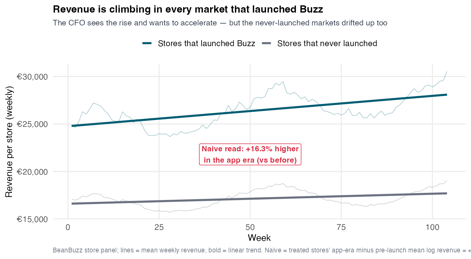
BeanBuzz rolled its loyalty app out market by market: every launched market’s revenue climbs after go-live, and the memo asks — accelerate the rollout?

Outcome \(Y\) = log weekly revenue → effects read as percent; higher is better — the opposite of last assignment’s cost outcome.

The seductive read — each market’s revenue after the app vs before — books +16.3%. It is also wrong, and the rest of the session is why.

Meet the running example and spring the CFO trap in one beat. BeanBuzz is a coffee chain rolling out a loyalty app across 40 regional markets in five waves; the CFO’s chart looks like a slam dunk — average revenue in launched markets rises steadily after each launch — and the high-stakes question is whether to accelerate the remaining waves. The whole session is the answer: the chart cannot tell you, because of how the rollout was sequenced.

Housekeeping to flag once (folded onto this slide): the outcome is revenue on a log scale, so every estimate reads as a percentage change, and the sign convention is that higher is better — the app’s true effect is positive. That is the opposite of the cost-outcome students saw in the prior assignment, where lower was the win; say it once and keep the direction straight, because when we later call TWFE “biased toward zero” that means biased DOWNWARD from +4.9%.

Now the trap: a naive before-versus-after on the treated markets gives +16.3% on log revenue — a huge, seductive figure, and it is wrong. A pre/post comparison attributes to the app everything else that changed between the two periods — winter seasonality and the secular macro trend that lift every market, launched or not; there is no control for “what would have happened anyway.” The +16.3% is the anchor we demolish in stages: naive +16.3% overstates wildly, static TWFE +3.7% corrects most of it but is biased, and the robust family lands near +3-4% against a true ATT of +4.9%. By the end, students should viscerally distrust any unadjusted pre/post number.

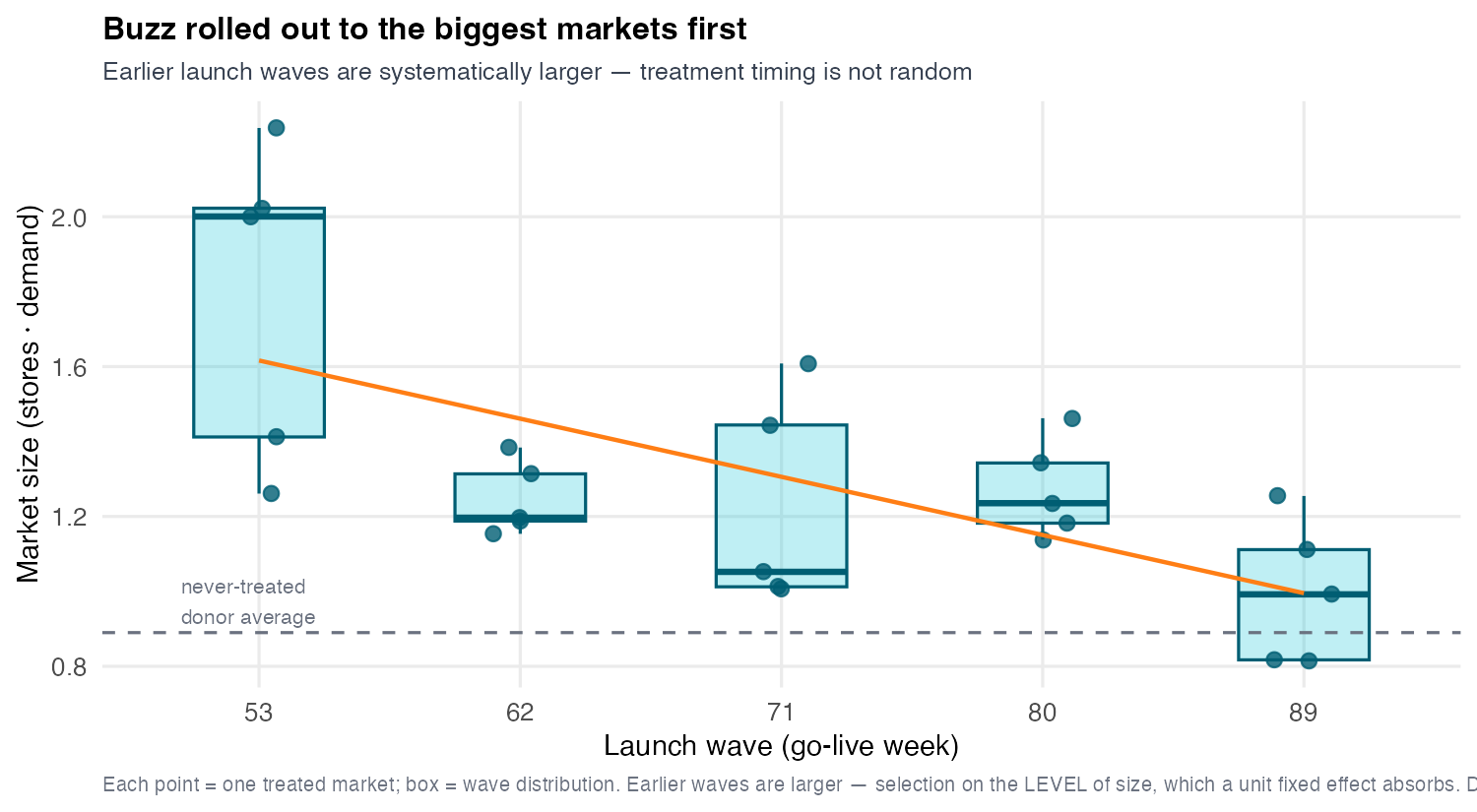
Buzz launched in its biggest markets first

The rollout was not random — the biggest markets went first. That is selection on the level of size, which a unit fixed effect absorbs. What would break DiD is selection on the trend — and this rollout avoids it.

Two distinct points, and keeping them separate is the whole craft. First, the naive +16.3% is inflated by time, not selection: a treated-only pre/post books everything that moved between the two windows — the gentle secular uptrend and the coffee-seasonality that peaks in winter (the post-launch windows sit near the week-56 peak). Decomposed against the known truth, the naive +16.3% = +11.4pp of pure counterfactual time + the true +4.9% app effect; of that +11.4pp, the secular uptrend contributes ≈ +4.4pp and the winter seasonality plus other common movements ≈ +7pp. The app’s own ramp is the +4.9%, not part of the inflation. A market’s constant level — big or small — is present in both the pre and the post window, so it cancels in a within-market before/after; selection on size does not inflate the naive.

Second, then, why show the rollout at all? Because it tells you which control is legitimate. The app went to the biggest markets first, so treated and never-treated markets differ in level — you cannot compare raw levels, you need a control whose trend the treated markets share. That is exactly what parallel trends buys, and a unit fixed effect removes the size gap for free. The bias a DiD cannot survive is selection on the trend — rolling out precisely where growth was already accelerating — because no unit fixed effect can subtract a slope. Here the rollout selected on level, not trend, so parallel trends is plausible; flag that this is the assumption the rest of the session leans on, and the one Assignment V makes you stress-test when a cohort violates it.

Subtract the trend they would have had anyway

The whole method, compressed

Subtract the common time trend the control would have had anyway. What’s left is the app’s effect.

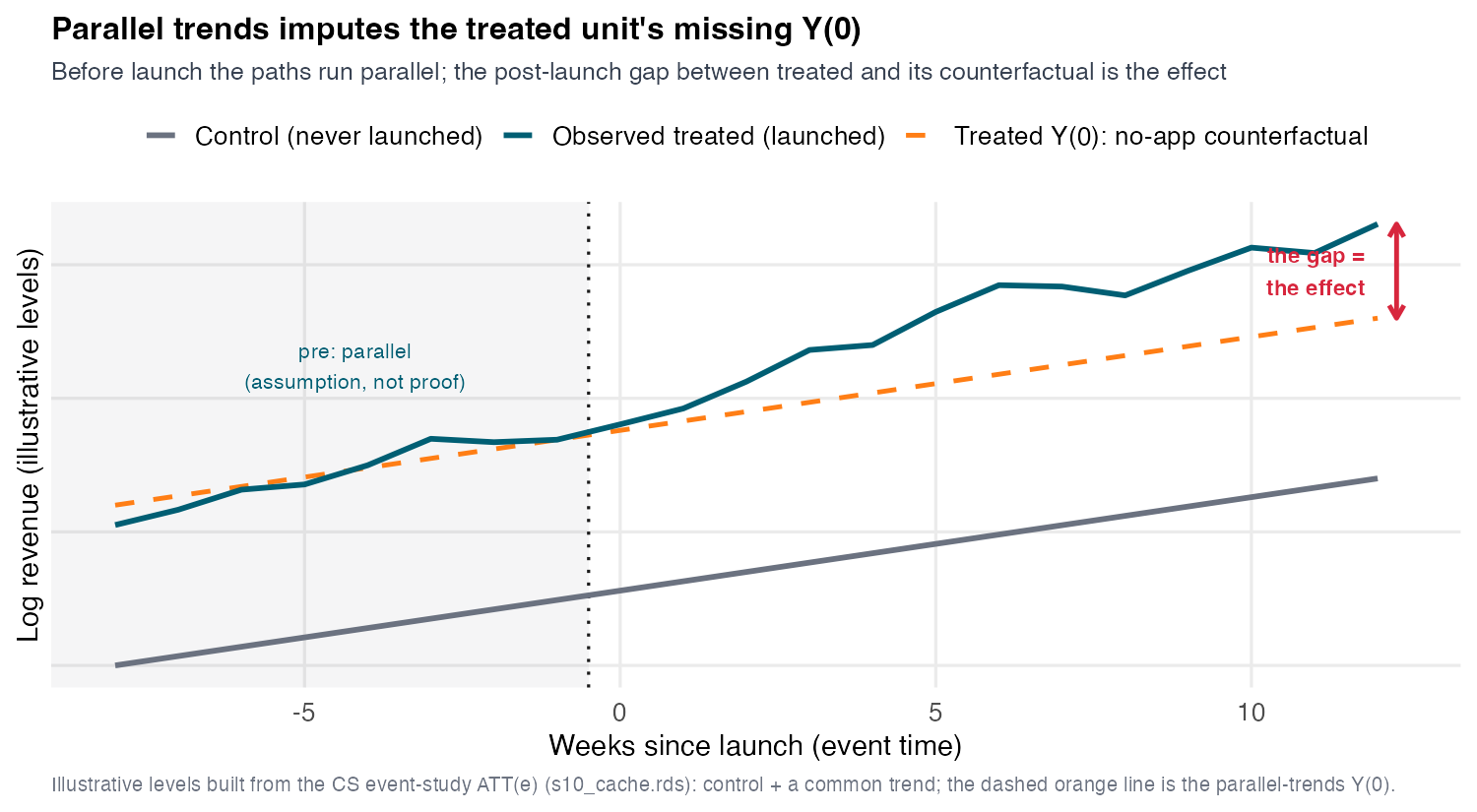
That subtraction is an imputation of the missing Y(0): we fill each treated market’s unseen no-app path using markets that didn’t (yet) get the app.

The Part V spine: impute the missing Y(0) under escalating assumptions. S10 uses additive unit + time effects — exactly the parallel-trends assumption. S11 relaxes it (synthetic control); S12 generalizes it (counterfactual imputation).

This is the thesis slide — the one sentence to carry through the whole deck. Difference-in-differences subtracts the counterfactual trend (what the treated markets would have done without the app) from their observed trend; the residual is the causal effect. Reframe that subtraction as imputation, because that is the Part V spine: we are filling the blanked-out Y(0) block for treated-and-post observations, and DiD fills it with an additive unit-plus-time model — each treated market’s no-app path equals its own level plus the common time trend estimated from untreated markets. That additive structure IS parallel trends. Give students the image to hold for the whole of Part V: a spreadsheet with a blanked-out rectangle — the never-observed Y(0) for treated markets after launch — that we impute under escalating assumptions across three sessions. Plant the three-session arc now: S10 imputes with additive effects (parallel trends), S11 with a weighted match (synthetic control), S12 with a flexible factor model (counterfactual imputation). Same missing block, escalating assumptions.

Basic 2×2 Model

Start with two markets and four numbers

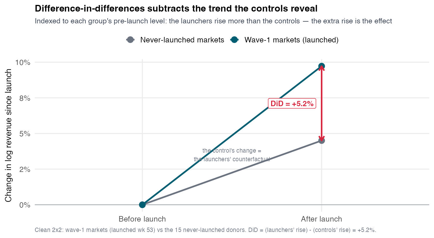
Strip it to the bone: the wave-1 launchers, the never-launched markets, two periods. Four cell means — that’s the entire engine.

Build intuition on the smallest possible case before scaling to the staircase. Take one early-treated market and one never-treated donor market, observe each in a pre-launch and a post-launch period, index both to 100 in the pre-period. That gives four numbers — the four cell means — and the entire DiD method is an arithmetic operation on those four numbers. Everything more elaborate (staggered timing, covariates, the robust estimators) is built by aggregating cases exactly like this one. The figure previews the punchline: the wave-1 market vs never-treated donor gives a clean DiD of +5.2%, the early-cohort effect. Keep this 2x2 concrete and visual; the next slide diagnoses why one market can’t do it and brings in the control, then the formula slide just names what the picture already shows. Note: this is the early-cohort number, not the overall ATT — do not conflate them.

The jump confounds two things — the control isolates one

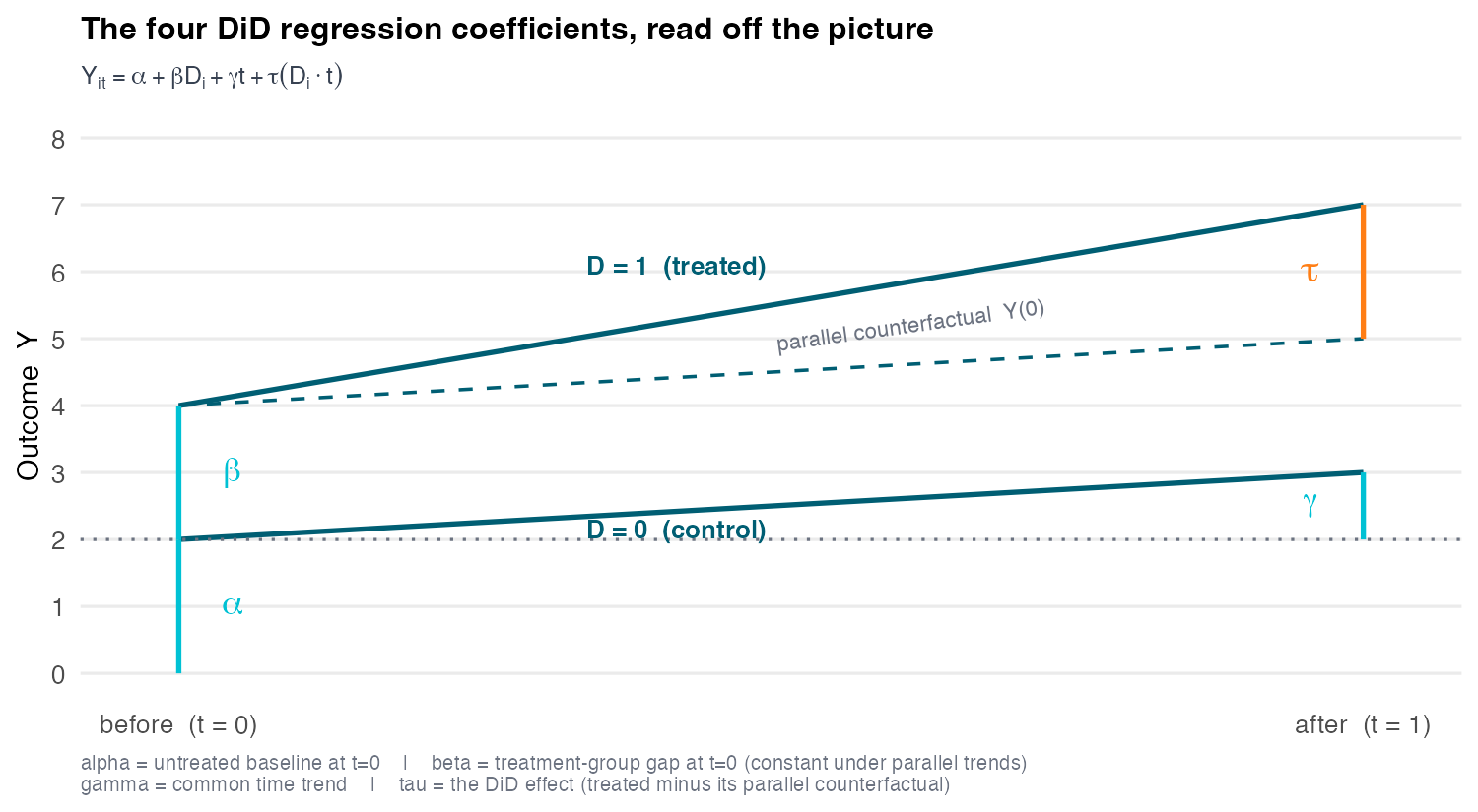
Look only at the treated market: its pre-to-post jump bundles two movements one market can’t separate — the app’s effect and everything else (winter seasonality, the macro trend that lifts every market). It’s the +16.3% mistake in miniature.

The never-treated donor got no app — so its pre-to-post change is pure time. Borrow it:

The borrowed counterfactual

We assume the treated market would have moved by the same amount as the control absent the app — so the control’s \(\Delta\) is the treated market’s unseen Y(0) trend.

One slide, two beats: diagnose the single-market comparison, then resolve it with a control. First the problem — the treated market’s pre-to-post jump is a sum of the app’s causal effect and a time effect common to everyone (seasonality, the macro environment, the market’s own trajectory); with data from only the treated market you cannot decompose the jump, the time effect and the treatment effect are perfectly entangled. It is the CFO’s +16.3% error shrunk to one market. That is precisely why a control is indispensable — not to match levels, but to estimate the common time movement so it can be netted out.

Now the resolution. Because the donor never received the app, its entire pre-to-post change is the common time effect — seasonality plus macro plus trend, with no treatment component. DiD’s identifying move is to borrow that change: assume the treated market would have experienced the same time effect absent the app, so the control’s delta is our estimate of the treated market’s unseen no-app delta. This is the imputation of Y(0) made fully concrete — we are not observing the treated market’s counterfactual, we are filling it with the control’s observed trajectory. Emphasize that the assumption is about the CHANGE (the trend), not the LEVEL: the two markets can sit at very different revenue levels and DiD is still valid, as long as they would have moved in parallel. That distinction is the whole content of parallel trends, and the next slide turns it into the estimator formula.

DiD = the jump minus the trend it would have had

Subtract the control’s change from the treated market’s change:

\[\widehat{\text{DiD}} \;=\; \underbrace{(\bar Y^{\text{treat}}_{\text{post}} - \bar Y^{\text{treat}}_{\text{pre}})}_{\text{treated jump}} \;-\; \underbrace{(\bar Y^{\text{ctrl}}_{\text{post}} - \bar Y^{\text{ctrl}}_{\text{pre}})}_{\text{time alone}}\]

The second term is the imputed Y(0) trend. What survives the subtraction is the app’s effect, free of the common time movement.

On the wave-1 launchers vs the never-launched markets: DiD = +5.2% — far below the naive +16.3%.

The early-cohort building block — not the portfolio-wide ATT, which the robust estimators pin near +3.3% once all cohorts pool (the robust menu).

The estimator in one line, and the reveal of how much the naive number was inflated. The double difference subtracts the control’s change (the time effect) from the treated market’s change (treatment plus time), leaving the treatment effect. Read the second term aloud as “the imputed Y(0) trend” to reinforce the Part V framing — the control’s change is literally the counterfactual we plug in for the treated market’s missing no-app path. On this 2x2, the early-cohort DiD is +5.2%, dramatically smaller than the +16.3% naive read: roughly two-thirds of the apparent effect was the common time movement — secular trend and seasonality — that every market, treated or not, would have seen anyway. Stress that +5.2% is the WAVE-1 number (early cohorts, biggest markets) — it is a clean building block, not the portfolio-wide ATT, which the robust estimators will pin near +3-4% once all cohorts are pooled.

The whole method rests on one claim: parallel trends

DiD is valid iff the treated market would have tracked the control absent the app — the dashed Y(0) path. Parallel trends is the assumption you must defend — no-anticipation and no-interference ride along (stated shortly).

Two separate jobs, done in order: first get a credible number, then interrogate this assumption. We can’t test it directly, so we save it for last.

This is the identifying assumption, stated as starkly as possible. DiD identifies the ATT if and only if the treated units would have followed a path PARALLEL to the controls had they not been treated — that is the dashed counterfactual Y(0) line in the figure. Everything rides on this one claim, and it is fundamentally untestable: we never observe the treated market’s no-app path after launch, so we can never confirm parallel trends directly. Note what the assumption does and does not require: it does NOT require equal levels (the lines can start far apart), only equal trends (the same slope absent treatment). It also depends on the functional form — parallel in levels is a different assumption than parallel in logs — which is why we work in logs throughout and flag it. Set up the session’s two-part structure explicitly here: these are two DISTINCT problems, and we tackle them in order. First, even GRANTING parallel trends, staggered timing breaks naive TWFE estimation — that is a mechanical estimation issue, not an identification one, and we fix it with the robust menu to get a credible number. Only then do we come back to interrogate parallel trends itself — the event-study diagnostic and the HonestDiD sensitivity. Estimate first, interrogate second; do not let the two issues blur together.

The estimand: the effect on the treated, after launch

DiD targets the Average Treatment Effect on the Treated (ATT) — the app’s effect on the markets that actually launched, in the periods after they did:

\[\tau_{\text{ATT}} \;=\; \mathbb{E}\big[\,Y_{it}(1) - Y_{it}(0) \,\big|\, \text{treated, post}\,\big]\]

Why the ATT and not the ATE? Because DiD asks for less. The ATE would need full unconfoundedness — treated and control comparable on both potential outcomes. DiD needs only the treated group’s untreated path to be borrowable — a one-sided condition on \(Y(0)\).

Weaker ask, narrower answer

Randomization buys the ATE. DiD trades it for the ATT — a narrower estimand — in exchange for the weaker, one-sided parallel-trends assumption you can actually defend. It is the unconfoundedness of S06–S09, moved from levels to changes.

Name the estimand explicitly — the deck has used “ATT” throughout without ever defining it, so define it here. The ATT is the average treatment effect on the treated: the effect of the app on the markets that launched, averaged over their post-launch periods — not the effect on a random market. Contrast it sharply with the ATE. Why does DiD target the ATT, not the ATE? Because the ATE would require full unconfoundedness — treated and control comparable on BOTH potential outcomes — which is what randomization delivers and an observational rollout does not. DiD asks for strictly less: it needs only the treated markets’ counterfactual UNTREATED path to match what the controls reveal — a one-sided condition on Y(0) alone. That one-sided ask IS parallel trends, and it is the same ignorability idea from S06–S09, moved from the LEVEL of Y to the CHANGE in Y. That is the bridge back to the course’s identification scaffolding: DiD is not a new philosophy, it is unconfoundedness-in-differences. The narrower estimand is the price of the weaker assumption.

Three assumptions, stated once

Parallel trends does the heavy lifting — but it is not alone. DiD identifies the ATT under three:

(A1) Parallel trends

\(\mathbb{E}[\,Y_{\text{post}}(0){-}Y_{\text{pre}}(0)\mid \text{treated}\,] = \mathbb{E}[\,Y_{\text{post}}(0){-}Y_{\text{pre}}(0)\mid \text{control}\,]\) — absent the app, the two groups would move in parallel.

(A2) No anticipation

No effect before launch: \(Y_{\text{pre}}(1){=}Y_{\text{pre}}(0)\) for the treated. This is what lets a not-yet-treated market stand in as a clean control.

(A3) SUTVA / no interference

One market’s launch doesn’t move another’s revenue — no spillover. In a geo-rollout, the live threat to watch.

Give the three identifying assumptions a formal home — the deck leaned on parallel trends alone, but two more are doing silent work. (A1) Parallel trends: absent treatment, treated and control would have the same change in Y(0) — the assumption everything visibly rides on. (A2) No anticipation: treated units show no effect before launch, so their pre-period outcome is a clean Y(0); this is precisely what licenses using a not-yet-treated market as a control (the whole Callaway-Sant’Anna move). Without it, “not yet treated” would already be contaminated. (A3) SUTVA / no interference: one market’s launch does not change another market’s revenue. In a geographic rollout this is a genuine, live threat — cannibalization or brand spillover across neighbouring markets would violate it — so name it rather than assume it away. Parallel trends is the one you must DEFEND with evidence; no-anticipation and no-interference are maintained assumptions you must be able to ARGUE. When we read the event-study leads later, note that flat leads are evidence for parallel trends AND no-anticipation jointly — they probe both.

Why the double difference works

The estimator is a theorem, not a heuristic — each step licensed by an assumption:

\[ \begin{aligned} \tau_{\text{ATT}} &= \mathbb{E}[\,Y_{1}(1) - Y_{1}(0)\mid D{=}1\,] \\[2pt] &\overset{\text{(A2)}}{=} \underbrace{\mathbb{E}[Y_{1}\mid D{=}1] - \mathbb{E}[Y_{0}\mid D{=}1]}_{\text{treated change (observed)}} \;-\; \mathbb{E}[\,Y_1(0){-}Y_0(0)\mid D{=}1\,] \\[2pt] &\overset{\text{(A1)}}{=} \big(\mathbb{E}[Y_1\mid D{=}1] - \mathbb{E}[Y_0\mid D{=}1]\big) - \big(\mathbb{E}[Y_1\mid D{=}0] - \mathbb{E}[Y_0\mid D{=}0]\big) \end{aligned} \]

(A2) adds and subtracts the treated group’s pre-period; (A1) swaps its unseen \(Y(0)\) change for the control’s observed one. Consistency turns each \(Y(\cdot)\) into an observable mean — the double difference.

Walk the derivation slowly — it is three lines and it shows the estimator is a theorem, not a plausible-looking recipe. Start from the definition of the ATT: expected Y(1) minus Y(0) for the treated in the post period. Line two uses no-anticipation to add and subtract the treated group’s pre-period outcome, splitting the expression into the treated group’s OBSERVED change (post minus pre, both realized) minus the treated group’s unobserved counterfactual change in Y(0). Line three is where parallel trends earns its keep: it lets us replace the treated group’s unseen Y(0) change with the CONTROL group’s observed change — because under parallel trends those two changes are equal in expectation. What survives is the double difference: (treated post minus treated pre) minus (control post minus control pre). Consistency/SUTVA is the quiet step that lets us write each potential outcome as the realized, observed mean. So the +5.2% we computed by hand earlier is not an analogy — it is this identity evaluated on four cell means. This is the old deck’s identification proof, kept because a Master-level audience should see WHY the arithmetic is causal, not just that it is.

The 2×2 as a regression — repeated cross-sections too

\[Y_{it} = \alpha + \beta\,D_i + \gamma\,t + \tau\,(D_i \times t) + \varepsilon_{it} \qquad (\alpha\text{ baseline},\ \beta\text{ group gap},\ \gamma\text{ trend},\ \tau=\text{DiD})\]

• Needs no panel — works on repeated cross-sections (different customers, houses, or visits sampled before and after).
• On a panel, unit + period fixed effects absorb \(\alpha{+}\beta D_i\) and \(\gamma t\), collapsing it to \(Y_{it}=\alpha_i+\lambda_t+\tau D_{it}\) — the TWFE form we build on next, whose lone slope is this same \(\tau\).

Turn the picture into the estimator, and make two points the old deck made that the narrative version dropped. First: the interaction regression Y = alpha + betaD + gammat + tau(D x t) reads the whole 2x2 off four coefficients — alpha is the untreated baseline at t=0, beta is the treatment-group gap at t=0 (which must be CONSTANT for parallel trends to hold — that is beta’s role), gamma is the common time trend, and tau, the interaction coefficient, is the DiD effect itself. The sketch labels each as a segment. Second, the reason this form matters beyond the panel: it identifies the DiD on REPEATED CROSS-SECTIONS — different units sampled before and after (survey waves, different houses listed pre- and post-highway, different customers) — where you cannot use unit fixed effects because no unit appears twice. That is a genuinely different data structure from our BeanBuzz panel, and the interaction OLS is what covers it. Finally, the panel-vs-cross-section reconciliation: on a PANEL, the unit fixed effects absorb alpha + betaD and the period fixed effects absorb gammat, so the interaction OLS collapses to the two-way fixed-effects form Y = alpha_i + lambda_t + tauD_it — exactly the TWFE regression the next act opens with, carrying the SAME tau. The main effects (alpha, the group term betaD, gammat) are what the unit and period fixed effects swallow; the interaction survives as the lone slope, and we write it tau in both places — the same treatment-effect letter as S08’s DML, and the same D for the treatment indicator. The one caveat students should hold: the group indicator D_i (a unit is in the treated group) times the post dummy t equals the treated-and-post cell indicator D_it — same D, the interaction is just its product with time.

With one launch date, the 2×2 scales to full dynamics

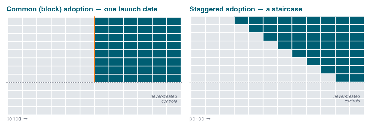
Nothing forces just two periods. If every treated unit launches on the same date (common / block adoption — left), the 2×2 scales up:

• Static TWFE stays a clean DiD — one launch date ⇒ no already-treated-as-control comparisons; extra periods just sharpen it.
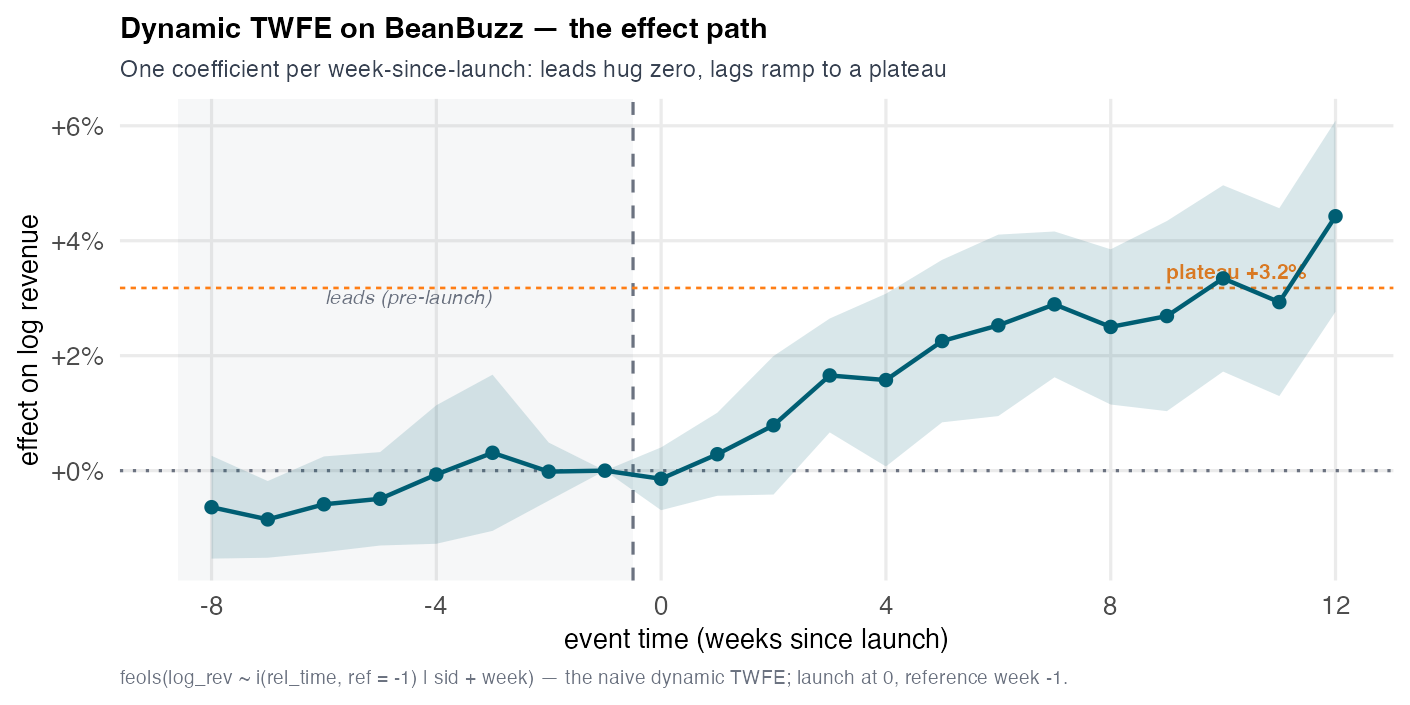
• Dynamic TWFE — one coefficient per period-since-launch — traces the effect path (leads ≈ 0, lags = the ramp):

\[Y_{it} = \alpha_i + \lambda_t + \textstyle\sum_{k \neq -1} \beta_k\,\mathbf{1}[\,t - g = k\,] + \varepsilon_{it} \qquad (g\ \text{shared by all treated})\]

The catch: one shared date. Real rollouts stagger it (right) — and that breaks TWFE.

The bridge from the 2x2 to the staggered problem, and the natural first home for the event study. Three beats. (1) The canonical 2x2 used two periods, but nothing requires that — only a single COMMON adoption date. If every treated unit launches on the same date (common or “block” adoption, the left schematic), the panel can have as many periods as you like and static TWFE, Y = alpha_i + lambda_t + tau*D_it, is STILL an unbiased, clean DiD: with one launch date the only comparisons TWFE ever forms are treated-vs-not-yet-treated and treated-vs-never-treated, so the forbidden comparison that wrecks staggered TWFE simply cannot arise. Extra periods just buy precision. (2) More periods hand you something new for free: replace the single treatment dummy with one coefficient per period-since-launch and you recover the DYNAMIC treatment effect — the event study. Leads (k<0) should hover near zero; lags (k>0) trace the ramp-to-plateau. Emphasize g is COMMON to all treated units here. (3) The transition, which is the whole point of the slide: everything here rests on that single shared date. Real rollouts stagger adoption across units — the right schematic, exactly the BeanBuzz staircase — so g becomes unit-specific g_i. That one change, timing VARIATION, is what breaks naive TWFE (the forbidden comparisons of the next act) and, later, contaminates this very event study (Sun-Abraham, in the parallel-trends act). So the slide plants two things the rest of the session cashes out: the estimator (dynamic TWFE / event study) we reuse as a pre-trend diagnostic, and the precise culprit — it is the variation in timing, not the number of periods, that breaks everything.

Staggered Adoption

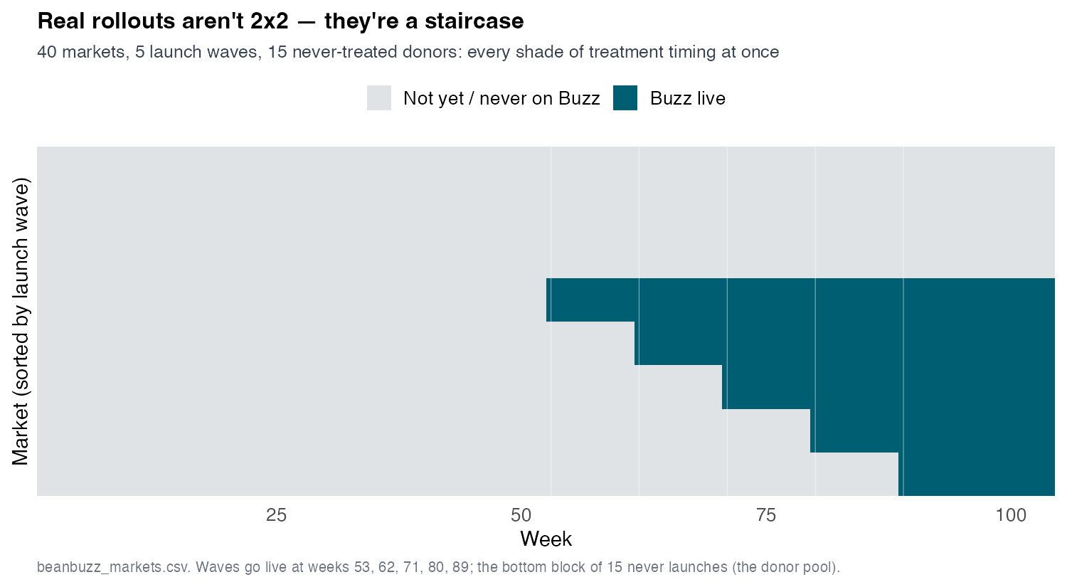
Real rollouts aren’t 2×2 — they’re a staircase

BeanBuzz: 233 stores, 40 markets, 104 weeks. Five launch waves at weeks 53/62/71/80/89, plus 15 never-treated donor markets. Timing varies — the clean 2×2 is gone.

Scale up from the toy 2x2 to the real design and let the structure sink in. BeanBuzz is a panel of 233 stores in 40 markets over 104 weeks. The app launches in five staggered waves — weeks 53, 62, 71, 80, 89 — and 15 markets never get it, serving as clean donor controls throughout. The figure’s staircase is the defining feature: at any given week some cohorts are already treated, some are about to be, and some never will be. This staggered structure is what breaks the tidy 2x2 and, as the next slides show, what breaks naive TWFE. The 15 never-treated markets are precious — they are uncontaminated controls available at every point in time, and the robust estimators will lean on them heavily. Anchor these numbers; the lab rebuilds estimates on exactly this panel and students will see 233/40/104 again.

The instinct: throw it all in one TWFE regression

The two-way fixed-effects model — the regression form of the 2×2 arithmetic — now on the full staggered panel:

\[Y_{it} \;=\; \alpha_i \;+\; \lambda_t \;+\; \tau\,D_{it} \;+\; \varepsilon_{it}\]

• \(\alpha_i\) — market FE (differences out the level) · \(\lambda_t\) — period FE (differences out common time) · \(\tau\) — the DiD.
• With one treated group and two periods, \(\hat\tau\) equals the hand-computed 2×2 exactly. That equivalence is comforting — and, as we’ll see, dangerously misleading once timing varies.

feols(log_rev ~ i(treated) | sid + week, data = panel)

It runs. It gives one tidy number:

static TWFE: +3.7%

Much smaller than the naive +16.3% — looks like a sober, corrected estimate. But it is biased, and not in a way you’d guess.

Show the natural move and the plausible-looking number it produces. The same TWFE specification that exactly recovered the 2x2 now runs on the full staggered panel with one line of fixest, and it returns +3.7% — far below the naive +16.3%, so it looks like a responsible, confound-corrected estimate, and most practitioners would stop here and report it. The trap is that +3.7% is BIASED, and biased in a subtle, non-obvious direction: it is dragged DOWNWARD, below the true +4.9%, by comparisons the model should never have made. The bias is not from omitted confounding in the usual sense — the fixed effects handle that — but from the mechanics of how TWFE combines the staggered 2x2s when treatment effects grow over time. The next slides dissect exactly why. The headline to set up: the fix is not a better-specified regression, it is refusing to make the forbidden comparisons in the first place.

Note the deliberate setup carried onto this slide: TWFE = the 2x2 DiD EXACTLY in the canonical one-treated-group, two-period case (alpha_i sweeps the level, lambda_t the common time effect, tau the double difference), which is why it became the reflexive default for panel data. Students should leave believing TWFE = DiD — so the betrayal on the staggered panel lands hard. The equivalence is special to the 2x2; the moment treatment timing VARIES, TWFE becomes a weighted average of many 2x2s, some of which should never be formed.

Dynamic TWFE turns one number into the whole path

Swap the single dummy for one per week-since-launch (\(k = t - g_i\), each unit’s own launch \(g_i\)): \[Y_{it} \;=\; \alpha_i + \lambda_t + \textstyle\sum_{k \neq -1}\beta_k\,\mathbf{1}[\,t - g_i = k\,] + \varepsilon_{it}\]

feols(log_rev ~ i(rel_time, ref = -1) | sid + week, data = panel)

Leads hug zero, lags ramp to a +3.2% plateau — the dynamics static TWFE hid inside one number. But it is the same naive estimator: each lag \(\beta_k\) crushes every cohort into one number per column, so its lags carry forbidden-comparison exposure (the far-horizon drift). Why the column-crush is dirty, and the fix, come next.

The dynamic counterpart of static TWFE — the payoff of the common-adoption slide, now on the STAGGERED panel. Make the parallel explicit: static TWFE put a single treatment dummy in the regression and returned one number, +3.7%. Swap that single dummy for a full set of event-time indicators — i(rel_time, ref = -1), one coefficient per week relative to each unit’s OWN launch g_i — and the identical TWFE machinery returns the whole effect PATH instead: leads (pre-launch) and lags (post-launch). Read it: the leads hug zero (encouraging for parallel trends, though we defer that reading to the diagnostic act) and the lags ramp to a plateau around +3.2% by event-week 8-12 — the dynamics static TWFE compressed into a single average. Then flag the honesty point hard: this is still the NAIVE estimator. Under staggered adoption its lag coefficients are weighted sums that can borrow already-treated cohorts (Sun-Abraham), the same forbidden-comparison contamination that biases static TWFE. On BeanBuzz it is mild — it shows up as the slight drift above the plateau at the far horizon (event-week 12) — but it is the same failure mode, so we do NOT lean on these naive lags. The next slides dissect why (Goodman-Bacon, forbidden comparisons); the robust menu returns the trustworthy dynamic path (the Callaway-Sant’Anna dynamic aggregation), and we re-read these very leads as a pre-trend diagnostic in the parallel-trends act. So this slide shows what static TWFE hid, using the exact estimator the common-adoption slide introduced, and hands the bias question straight to the next slide. Two seams to manage if a sharp student presses. First, do NOT reconcile +3.7% (the pooled static number on the previous slide) with this +3.2% plateau arithmetically — a pooled TWFE is not the time-average of this path (the ramp starts near zero), and that very mismatch is the Goodman-Bacon weighting point the next slides dissect. Second, the contamination’s SIGN need not be uniform: forbidden comparisons drag the POOLED static estimate DOWN (+3.7% below the true +4.9%), yet a terminal-horizon LAG here drifts slightly UP — the same weighting artifact, not a single-direction bias. And on this slide the drift is a flagged preview, not yet proof: it is confirmed as forbidden-comparison contamination only once we overlay the robust CS version in the parallel-trends act.

TWFE secretly averages every 2×2 it can build

Goodman-Bacon’s result: static TWFE is a variance-weighted average of all the 2×2 DiDs in the panel. (Goodman-Bacon 2021)

Some of those 2×2s are clean:

• treated vs never-treated ✓
• treated vs not-yet-treated ✓ (the future-treated are valid controls for now)

But to use every period, TWFE also builds a third kind — and that one is poison.

This is Goodman-Bacon’s decomposition, the analytical heart of the act. Static TWFE on a staggered panel is not estimating one thing — it is a variance-weighted average of every 2x2 DiD that can be constructed from the data, with weights proportional to group sizes and treatment-variance. Two of the three flavors of 2x2 are perfectly legitimate: early-treated vs never-treated (clean), and early-treated vs not-yet-treated (also clean, because a unit that will be treated later is a valid control while it is still untreated). If those were the only comparisons, TWFE would be fine. The problem is the THIRD flavor, which TWFE must form to exploit all the timing variation — using ALREADY-treated units as controls for LATER-treated units. That is the forbidden comparison, and it is the subject of the next slide. The decomposition is also a practical diagnostic: you can plot the 2x2s and their weights to see how much your TWFE leans on the bad ones.

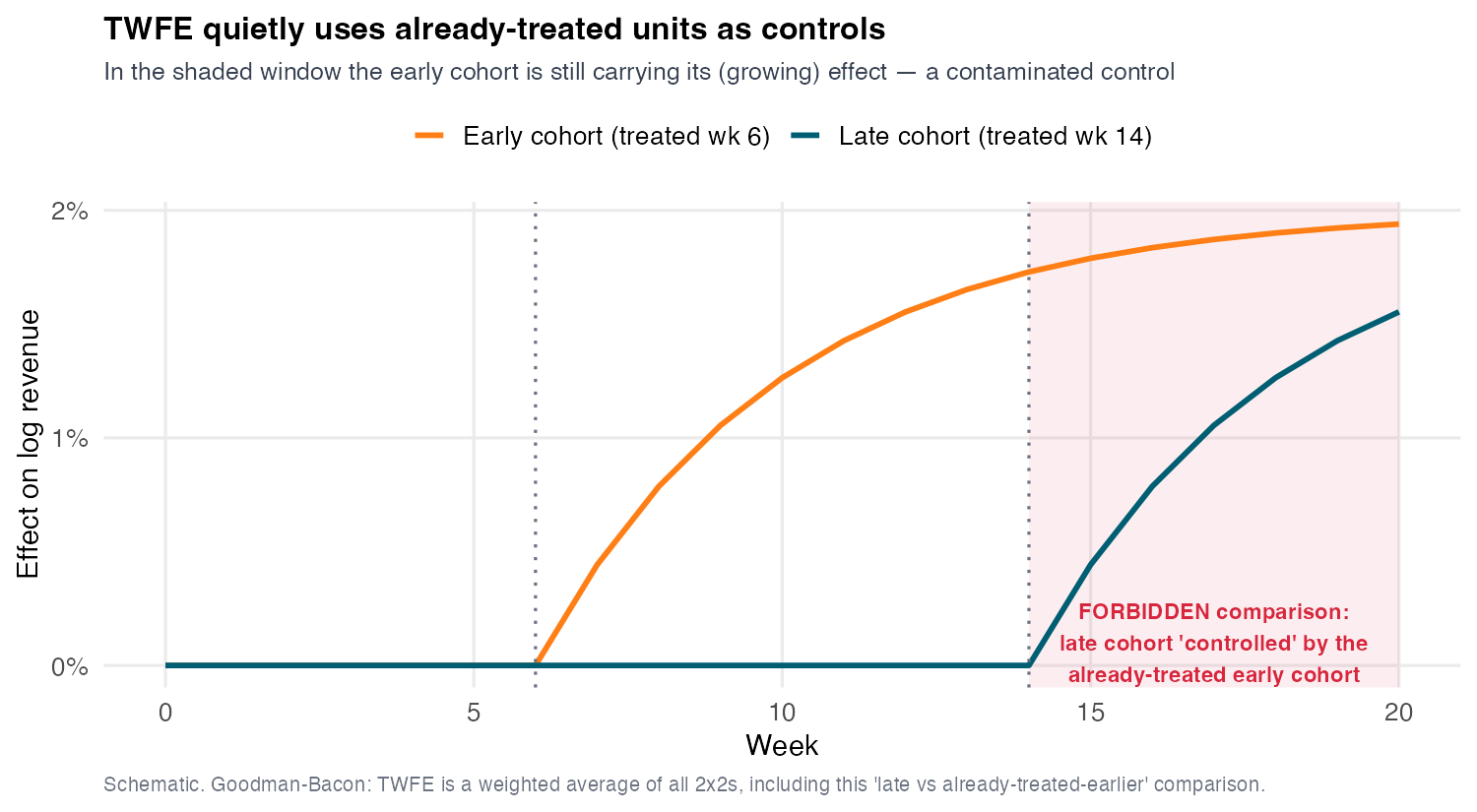
Using the already-treated as controls runs the clock backwards

The forbidden 2×2 uses an already-treated cohort as the control for a later cohort. But the control is still responding to its own treatment — so its change is not pure time. Subtracting it contaminates the estimate.

Make the forbidden comparison concrete and visceral. When TWFE uses an already-treated cohort as the control for a later-treated cohort, it implicitly assumes the already-treated cohort’s change over that window is pure time effect — exactly the role the never-treated donor played in the clean 2x2. But the already-treated cohort is STILL responding to its own app launch; if the effect grows over time (as BeanBuzz’s does, ramping to a plateau), the control’s outcome is rising for treatment reasons, not just time. Subtracting that rising path over-subtracts, and the later cohort’s estimated effect is pulled toward zero or even negative. The intuition “running the clock backwards” captures it: you are treating an outcome that already contains a maturing treatment effect as if it were a clean baseline. This is the mechanism behind the +3.7% being dragged below the true +4.9%.

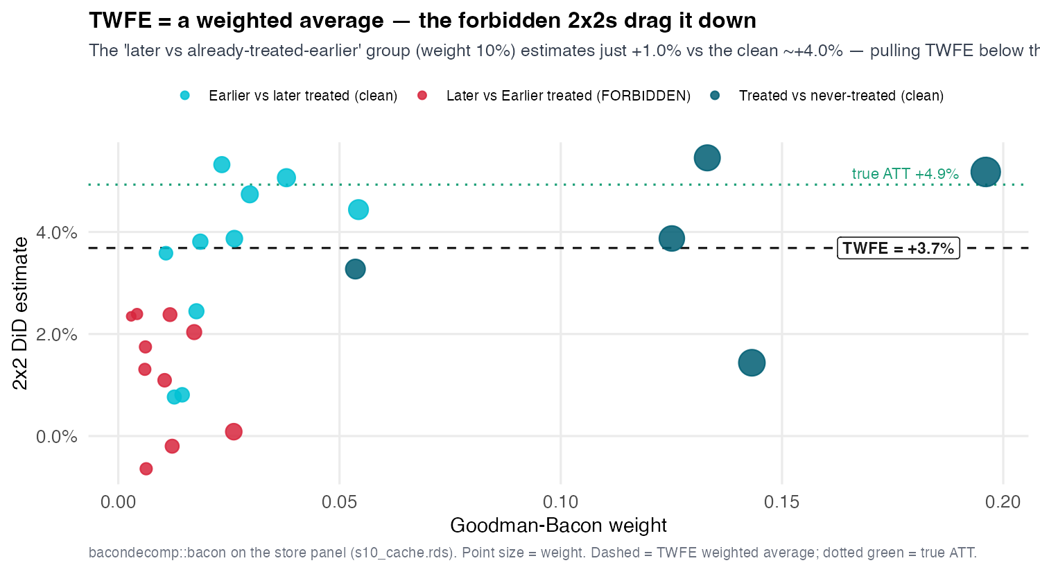
Goodman-Bacon shows where the weight goes

Plot each 2×2’s estimate against its weight. The clean comparisons cluster near +4.0%. The forbidden group sits low — near +1.0% — yet still carries ~10% of the weight.

The decomposition scatter turns the abstract result into a diagnostic you can read. Each point is one 2x2: horizontal position is its Goodman-Bacon weight, vertical position is its estimate. The clean comparisons — treated vs never-treated and treated vs not-yet-treated — cluster around +4.0%, close to the truth. The forbidden “already-treated as control” comparisons sit much lower, around +1.0%, because of the over-subtraction we just described, and critically they carry about 10% of the total weight. So TWFE’s +3.7% is a weighted blend that drags the honest ~+4% down toward the contaminated +1% — the forbidden group is a low-estimate anchor pulling the average toward zero. This plot is exactly what the lab produces with bacondecomp; students should learn to make it and eyeball how much of their TWFE rests on the low-estimate, forbidden cluster. The next slide states the general phenomenon and names the negative-weights result.

When effects grow, the forbidden weights turn toxic

The bias is worst exactly when the treatment effect grows over time — as BeanBuzz’s does (it ramps to a plateau).

• Here, the forbidden group is attenuated (+1.0% vs the clean +4.0%) and drags TWFE toward zero — the +3.7% is biased downward.
• In the general case, de Chaisemartin & D’Haultfœuille show these forbidden comparisons can receive outright negative weights — TWFE can even flip sign. (Chaisemartin and D’Haultfœuille 2020)

A weighted average where some weights are negative is not a treatment effect anyone asked for.

State the general pathology and calibrate the BeanBuzz-specific claim precisely so students do not overgeneralize. The bias is most severe when treatment effects are dynamic — growing over time — which is the realistic case and BeanBuzz’s case. Be careful with the framing: on BeanBuzz the forbidden group is ATTENUATED (its estimate is +1.0% versus the clean +4.0%) and that low value drags the weighted average down to +3.7%, biased TOWARD ZERO from the true +4.9% — a contaminated, attenuated estimate, not literally a negative weight in this dataset. The general phenomenon, due to de Chaisemartin and D’Haultfoeuille, is stronger: forbidden comparisons can receive outright NEGATIVE weights, and in extreme cases TWFE can even return the wrong sign. Distinguish these clearly — the deck’s honest claim is “biased toward zero / dragged down here; negative weights are the general worst case.” A weighted average with negative weights is not an interpretable causal quantity, which is the whole motivation for the robust menu.

The fix isn’t a better regression — two families, one rule

You cannot patch TWFE with controls or interactions — the problem is which comparisons it forms, not which variables it omits.

The principle that fixes everything

Never use an already-treated unit as a control — compare treated cohorts only to not-yet- or never-treated units. Forward-engineer the comparison; don’t reverse-engineer the regression. (Baker et al. 2025)

Every robust estimator enforces it, splitting into two families by how each builds the clean counterfactual:

• Family A — aggregate clean 2×2s: one clean treated-vs-control comparison per cohort, then average. → Callaway-Sant’Anna, Sun-Abraham.
• Family B — impute \(Y(0)\): model the untreated potential outcome, predict it for treated cells, average the gaps. → BJS, Gardner.

Deliver the constructive turn and the roadmap in one beat, briskly — every claim gets its own slide next. First the fix: TWFE’s failure is not an omitted-variable problem you can cure with more controls or fancier interactions — it is a problem of WHICH 2x2 comparisons the estimator forms, and no regression respecification cures a contaminated comparison set. The fix is a design principle students should memorize: never use an already-treated unit as a control; only compare treated cohorts to not-yet-treated or never-treated units. Baker et al. frame this as “forward-engineering” — decide the causal estimand and the clean comparisons FIRST, then derive the estimator, rather than running a regression and reverse-engineering what assumptions would make it valid. Then the roadmap: every robust estimator that follows is a disciplined way of enforcing that rule, and they fall into exactly two families. Family A (Callaway-Sant’Anna, Sun-Abraham) builds explicit clean two-by-two comparisons — treated cohort against never- or not-yet-treated controls — and aggregates them. Family B (Borusyak-Jaravel-Spiess, Gardner) never forms an explicit comparison; it models the untreated potential outcome Y(0), predicts it into the treated cells, and averages the realized-minus-predicted gaps. Do not evaluate any estimator here; this is scaffolding for the four slides that follow.

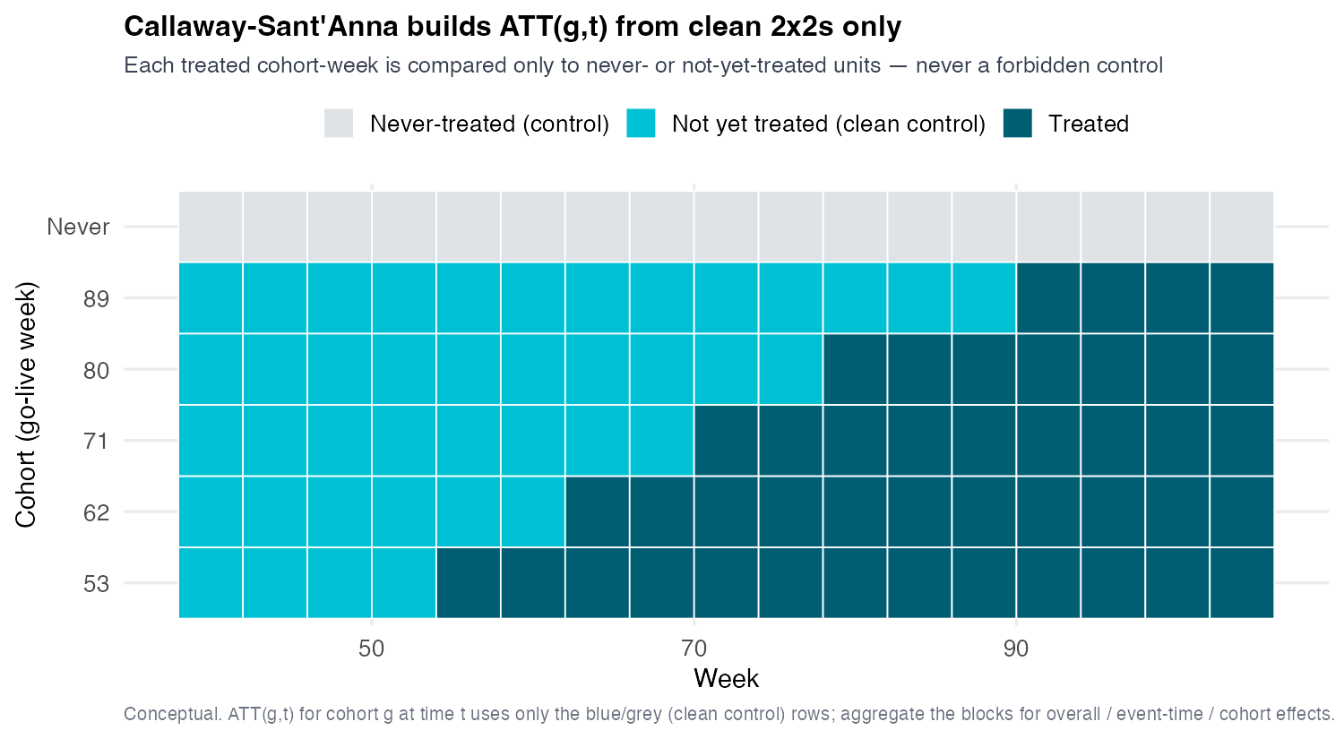
Callaway-Sant’Anna: don’t pool — one clean effect per cohort

Don’t pool. Estimate a group-time ATT — one clean effect per cohort \(g\), period \(t\), \(\text{ATT}(g,t)=\mathbb{E}[Y_t(g)-Y_t(0)\mid G=g]\) — identified as a transparent 2×2: (Callaway and Sant’Anna 2021)

\[\text{ATT}(g,t) = \mathbb{E}[\,Y_t - Y_{g-1}\mid G=g\,] \;-\; \mathbb{E}[\,Y_t - Y_{g-1}\mid \text{clean controls}\,]\]

= (cohort \(g\) change) − (not-yet / never-treated change)

Introduce Callaway-Sant’Anna as the spine estimator of the whole act, mirroring how S09 used the AIPW score as its spine. The core idea is disaggregation: instead of forcing one pooled coefficient — the TWFE mistake — estimate a separate clean effect for each cohort g and each post-period t, the group-time ATT(g,t). Read the identification off the board slowly: it is a plain two-by-two — the change for cohort g from its base period g minus one to period t, minus the same-window change for units that are clean at t (never-treated or not-yet-treated); that is the two-term structure the small caption spells out. Because the control pool is restricted to clean units, an already-treated cohort structurally cannot enter as a control — that is the greyed-out region in the schematic, and it is the design enforcement of the forbidden-comparisons principle, not a regression patch. Note the base period convention g minus one (shift to g minus two if you allow one period of anticipation). The next slide shows the payoff of having all these blocks: aggregation.

Same blocks, many reports — aggregation is a choice, not a new assumption

Identification happens once, at the block level. Re-weighting is a reporting choice — call aggte(cs, type=…) and read the field; each answers a different question, in a different shape:

Report — aggte() field	In general	For BeanBuzz	Output
Overall group$overall.att	The average effect?	App’s worth, all markets?	one number — +3.3%
By cohort group$att.egt	Early vs late adopters?	Same gain in every wave?	one per wave — +1% to +5%
By calendar time "calendar"	Does the period matter?	Bigger lift some weeks?	one per week — ≈0% → +5.6%
By relative time "dynamic"	How does it evolve?	Weeks until it matures?	event study — ramp to +3%

Overall and By cohort are the same aggte("group") call — the overall is just the size-weighted roll-up of the per-wave effects. Disaggregate first, aggregate later.

A separate type=“simple” gives a cruder single overall, +3.5% — it overweights earlier-treated waves (they have more post-periods), so CS report the group roll-up +3.3%.

Aggregation is where the building-block design pays off — the panel echo of S09’s “one score, many projections.” Once you hold the clean ATT(g,t)s, the report you want is just a re-weighting; no new identifying assumption is added, because identification already happened at the block level. The point the table makes: the four aggte types return DIFFERENT SHAPES, not four versions of one number. type=“group” gives the overall +3.3 percent (its overall.att, weights proportional to cohort size — the deck’s headline) AND, in the same call, the by-cohort breakdown: the five launch waves run from about +1 percent for the week-80 wave up to about +4.7 percent for the week-62 wave — NOT monotone in adoption time, so resist an “early adopters always gain more” story. type=“calendar” gives one effect per calendar week, rising from near zero just after the first launches to about +5.6 percent late, as more markets treat and effects mature (overall +3.2). type=“dynamic” gives the event study — one coefficient per week-since-launch, the ramp to a roughly +3 percent plateau with flat pre-launch leads. Two honesty notes. First, only the overall collapses to a single number; the payoff of disaggregating is that you keep every piece and pick the report your question needs. Second, a cruder type=“simple” overall averages all cells with group-size weights and reads +3.5 percent — it overweights the earlier, bigger cohorts (they contribute more post-periods), which is exactly why Callaway-Sant’Anna recommend the group-weighted +3.3 percent the deck carries forward; and the dynamic aggregation’s own equal-weighted single number is +2.2 percent only because it averages in the early ramp, so don’t quote it as a rival estimate — the effect is the ~+3 percent plateau.

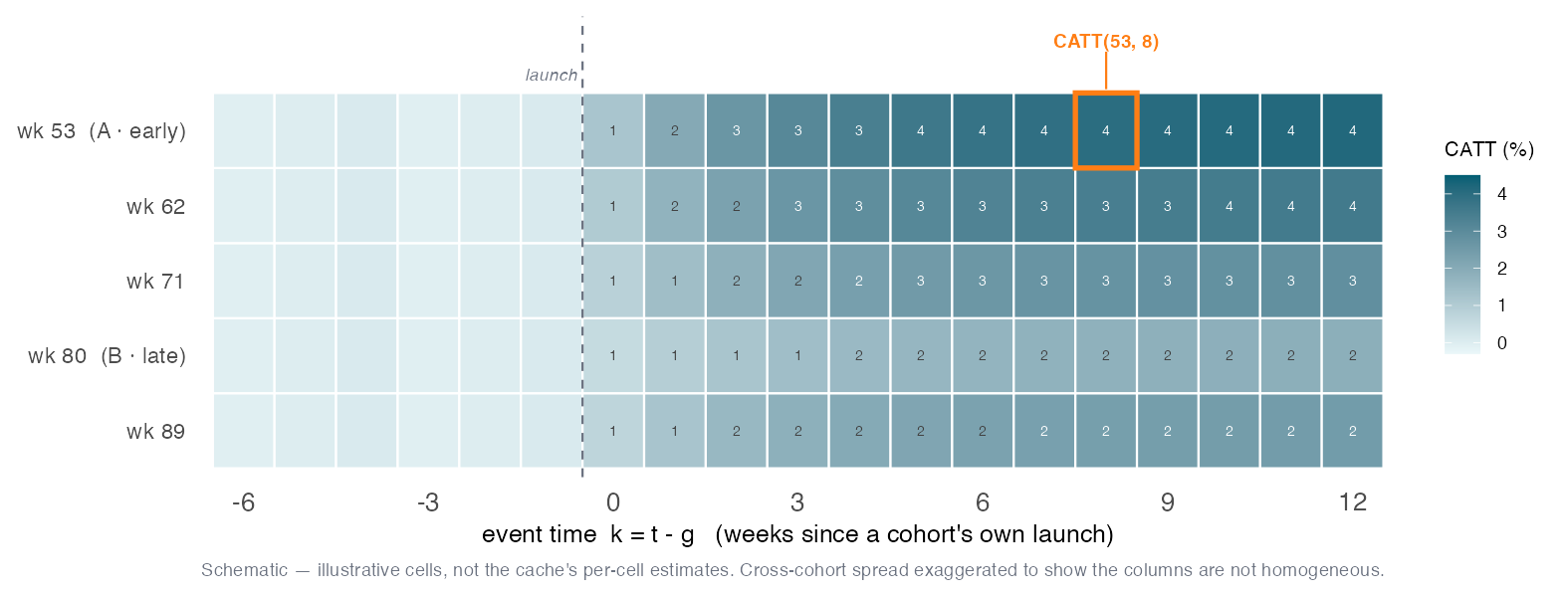
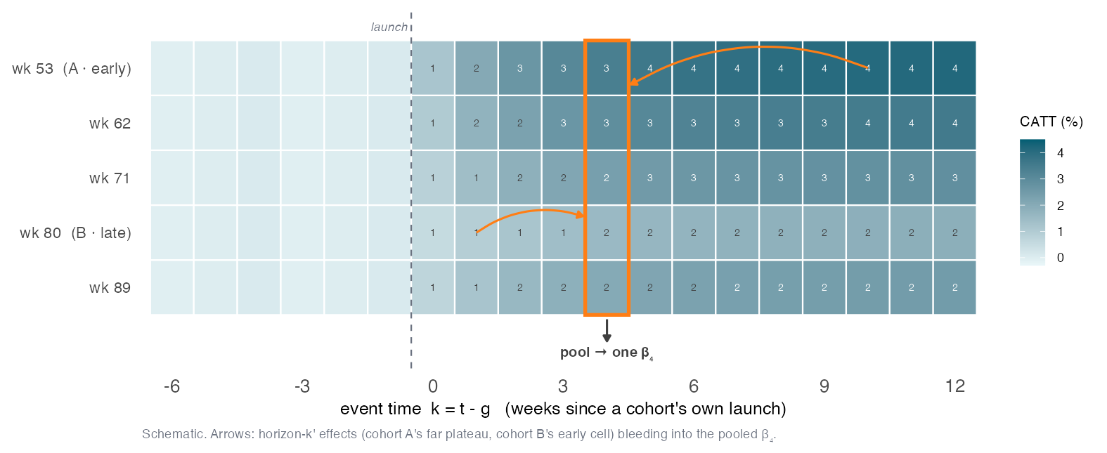
Every estimator reads the same CATT(g,k) grid

Line every cohort up by weeks since its own launch (\(k = t - g\)). One cell is the cohort average treatment effect on the treated — \(\text{CATT}(g,k)\), the number we actually want: (Sun and Abraham 2021)

\[\text{CATT}(g,k)\;=\;\mathbb{E}\big[\,Y_{g+k}(g)-Y_{g+k}(\infty)\,\mid\,G=g\,\big]\]

cohort \(g\)’s average effect \(k\) weeks after its own launch, against the never-treated baseline \(Y(\infty)\)

Set \(t=g+k\) and this is Callaway-Sant’Anna’s ATT\((g,t)\) read in event time — the same estimand, just estimated by a different clean control and fit (non-nested PT), so the cells need not match to the digit.

This slide fixes the “CATT introduced cold” gap: CATT is defined plainly, formulaically, AND visually before any contamination formula uses it. Read one cell slowly — CATT(g,k) is the average, over the markets that launched in wave g, of realized log-revenue minus the never-treated Y(infinity) baseline, k weeks after THAT wave’s own launch (Sun-Abraham Definition 1, re-indexed to (g,k)). The grid IS the definition: rows are cohorts, columns are weeks-since-launch, each cell is one CATT(g,k). Make it concrete with the two named waves we carry through the next slide: cohort A = the wk-53 wave (early), cohort B = the wk-80 wave (late); the highlighted cell is cohort A eight weeks after its launch. Then land the unifying anchor carefully: with t = g+k this is exactly CS’s ATT(g,t) re-indexed to event time — the SAME ESTIMAND (Sun-Abraham state this explicitly). Do NOT overclaim estimator/cell identity: SA and CS target the identical cell but use different clean controls (SA holds out never-/last-treated; CS can use not-yet-treated), different fits (one saturated OLS vs separate doubly-robust 2x2s), and non-nested parallel-trends assumptions — so the estimated cells need not coincide numerically. That is why SA’s +3.5% and CS’s +3.3% differ by construction, not by noise. The figure is SCHEMATIC (illustrative cells with exaggerated cross-cohort spread so the next slide’s column-crush reads as dirty) — the lab never materializes per-cell CATT; students run sunab(…) and read summary(sa, agg=‘att’) and iplot(sa). SA is cited here next to its definition and again where its saturated regression is introduced (the “same engine, saturated” slide).

Naive dynamic TWFE: the column-crush leaks

The naive event study forces one \(\beta_k\) per column, pooling every adoption cohort:

\[\beta_k \;=\; \underbrace{\textstyle\sum_g \omega_{g,k}\,\text{CATT}(g,k)}_{\text{column } k \text{ you wanted}} \;+\; \underbrace{\textstyle\sum_{k'\neq k}\sum_g \omega_{g,k'}\,\text{CATT}(g,k')}_{\text{leak from other columns}}\]

• Leak’s cause: cohorts’ effect heterogeneity (\(\text{CATT}(g,k)\) varies with \(g\)); if homogeneous, leak cancels.
• Leak’s vehicle: the two-way FE & the other event-time dummies mix cohorts at different maturities.
  • this sets the weights \(\omega\) — which can become negative → a coefficient sign flip.
  • leads also affected — a flat naive pre-trend plot is not a clean pre-trends test. (returns later)

This delivers the DISTINCT event-time contamination result — NOT a re-tread of Goodman-Bacon (the static forbidden-2x2 story is fully spent upstream; do NOT re-plot the bacon scatter). CATT is now warm from the previous slide, so the double-sum reads cleanly: beta_k is the column-k blend you wanted PLUS a leak from every OTHER column k’. Make the WHY visible, not asserted: to collapse one event-time column inside two-way FE, the regression nets cohorts sitting at DIFFERENT maturities against each other — point at the figure, where cohort A’s far-horizon plateau cell and cohort B’s early low cell both fall in the pooled column, so horizon-k’ effects bleed into beta_k. The implied weights are non-linear in the cohort mix and need not be positive, so a coefficient can flip sign. State the condition precisely (a common overclaim): dynamic-TWFE lags are fine when effects are heterogeneous ONLY in time-since-treatment; the pathology needs heterogeneity in the dynamic path ACROSS COHORTS (Sun-Abraham’s homogeneity assumption). One heuristic bridge you may say aloud to connect to the forbidden-comparisons rule — “this is the same never-use-an-already-treated-unit idea, now leaking across horizons” — but the LITERAL mechanism is correlation among the relative-period indicators plus the excluded/binned reference period, not the static 2x2; present the leak, not a derivation. Second consequence students miss (the crown-jewel SA result): the LEADS are contaminated too — a lead coefficient loads post-treatment CATT even with no anticipation, so a flat naive pre-period does NOT certify parallel trends; bold it, it returns in the parallel-trends act. On BeanBuzz the contamination is mild — the naive lags drift slightly above the robust CS path at the far horizon. The figure is schematic. This slide cashes the “still naive” flag raised on the dynamic-TWFE slide. Paper anchor (verified against Sun-Abraham Prop 2, the parallel-trends form): the estimand of beta_k is a weighted sum of CATT with weights that sum to +1 on the own relative period, 0 on each other included period, and -1 on the excluded/reference periods, and can be negative; the CATT form assumes parallel trends + no anticipation. The ROOT CAUSE the paper names is cross-cohort heterogeneity, NOT the fixed effects: under their Assumption 3 (CATT_{e,l} does not depend on cohort e) every contamination term cancels and beta_k = ATT_k, even though the two-way FE are unchanged. The FE + the other event-time dummies + the reference normalization are the VEHICLE that sets the weights (OLS/FWL residualization) — the on-slide “different maturities” line is that conduit. NB the slide folds SA’s two off-diagonal terms (other-included-periods + excluded-reference-periods) into one “leak from other columns,” and uses g=cohort/k=relative-time where SA use e=cohort/l=relative-time (their g is a bin of relative periods).

Same engine, saturated: cells, not columns

Sun and Abraham (2021) use the same dynamic TWFE engine, but saturate the grid with a cohort \(\times\) event-time interaction on the right-hand side and hold out control cohorts \(C\) (never-/last-treated):

\[Y_{it} = \alpha_i + \lambda_t + \textstyle\sum_{g\notin C}\sum_{k\neq -1}\delta_{g,k}\,\underbrace{\mathbf{1}[G_i=g]}_{\text{cohort } g}\,\underbrace{\mathbf{1}[t-g=k]}_{\text{event-time } k} + \varepsilon_{it}\]

	Naive dynamic TWFE	Sun-Abraham
Estimates	one \(\beta_k\) per event-time column — cohorts pooled	one \(\hat\delta_{g,k}=\widehat{\text{CATT}}(g,k)\) per cell
Control	none held out — \(\beta_k\) leaks other columns (\(\omega\) can be \(<0\))	each cell vs never-/last-treated only — no cross-cohort blend

Identification is done cell-by-cell — re-pooling the clean cells into a report is the last step, next.

This is the crisp side-by-side the professor asked for, now literally correct on the fixed effects. SAME feols engine, SAME two FE — alpha_i store (sid) + lambda_t week — the ONLY change is the right-hand side. Both specs are locked to sid+week to match the cache (make_s10_cache.R fits es_twfe and sunab both with | sid + week), so “same two FE, one interaction added” is true, not approximately true. i(rel_time, ref=-1) puts one beta_k per event-time COLUMN with all cohorts pooled (no control held out, column mixes maturities); sunab(ft_sa, week) saturates into one delta_{g,k} per cohort x horizon CELL, each estimated against the never-/last-treated control. Exact lab specs to say aloud (the clean forms stay on-face for continuity): the naive lab call is i(rel, ref = c(-1, -1000)) — the double reference drops the k=-1 base AND the never-treated sentinel bin; SA recodes the 15 never-treated markets to sentinel cohort ft_sa = 10000, which sunab uses as the last/never control. Honesty on “one interaction”: the reported +3.5% is NOT the raw saturated OLS output — the fix is three moves (saturate + hold the control cohort C out of the interactions + re-aggregate with cohort-share weights); this slide does the first two, aggregation is the next slide. The saturated equation sums g NOT in C, matching the “each cell vs never-/last-treated” row — the control cohorts carry no event-time dummies, so no forbidden cross-cohort blend can form. SA stays Family A, CS’s regression-native cousin — do not rank its PT above CS.

Clean cells in, any report out — the same spine as Callaway-Sant’Anna

Identification happened once, at the cell level — each SA coefficient \(\hat\delta_{g,k}\) is a clean \(\widehat{\text{CATT}}(g,k)\) cell. Pooling them back is a reporting choice, the same disaggregate first, aggregate later spine as CS:

SA report	How it pools the clean grid	Output
Event study \(\nu_k\) — iplot(sa)	within each horizon \(k\): cohort-share average across cohorts	ramp to a ~+3% plateau
Overall IW-ATT — summary(sa, agg="att")	one interaction-weighted average over the whole post-grid	+3.5%

\[\nu_k = \textstyle\sum_g \text{share}_{g,k}\,\widehat{\text{CATT}}(g,k),\qquad \text{share}_{g,k}\ge 0,\ \textstyle\sum_g \text{share}_{g,k}=1\]

\(\text{share}_{g,k}\) = cohort \(g\)’s fraction of the markets observed \(k\) weeks after launch (bigger cohorts count more). These non-negative shares replace OLS’s implicit possibly-negative weights — where the fix lives.

This gives aggregation real airtime, built as the deliberate mirror of the CS aggregation slide — same “identification happens once at the cell level; aggregation is a reporting choice, no new assumption” spine. Two shapes from the one clean grid. (1) EVENT-STUDY PATH nu_k: for each horizon k, average the clean cells ACROSS cohorts with cohort-share weights (each cohort’s share among cohorts observed at horizon k; non-negative, sum to one). Plotting nu_k against k is iplot(sa), the de-contaminated Sun-Abraham event study that ramps to the ~+3% plateau — this IS the “SA saturated version we built in the robust menu” the parallel-trends act calls back to. The contrast with the naive column-average, which used OLS’s implicit possibly-negative weights, is where the fix actually lives. (2) OVERALL number: summary(sa, agg=‘att’) returns +3.5% — an interaction-weighted average over the WHOLE post-treatment grid of clean cells, the SA analog of CS-SIMPLE, which is why the two land on 0.0350. CRITICAL — do NOT present the overall as an equal-weight average of the nu_k across horizons: equal-averaging the 0->~3% ramp is what gives CS its dynamic-OVERALL +2.3%, BELOW the plateau (the lab’s reflection Q1); the SA +3.5% overall is a whole-grid cell average, NOT the ramp-average, so keep +2.3% off this slide and never write IW-ATT = (1/|K|)*sum of nu_k. [Note: the exact internal weighting of summary(sa, agg=‘att’) was not read verbatim from fixest; +3.5% is the cache value (sunab$att = 0.0350), described verbally to avoid any formula-vs-number contradiction — worth a one-line cache check before final ship.] Load-bearing caveat to VOICE (the “Read the two headline numbers” callout was removed from the slide face — say this aloud): SA weights by cohort SHARE, CS’s headline by cohort SIZE; the +3.5% = CS-simple 0.0350 match is a dataset coincidence, not identity; CS’s carried headline stays +3.3%; keep the whole robust family (CS +3.3 / SA +3.5 / BJS +4.2 / Gardner +4.2) BELOW true +4.9%. Students run summary(sa, agg=‘att’) for the number and iplot(sa) for the path; they never hand-build the cohort-share average, so present the nu_k formula as the concept sunab executes internally.

Imputation: fit white, predict grey — at the strongest PT price

BJS (2024) and Gardner (2022) share one idea — model \(Y(0)\) where it is observed, then predict it where it is missing:

market × week panel

never-treated
early cohort
late cohort

week →

observed → fit white    missing → predict grey

1. Fit white — on the observed cells, estimate the additive \(Y_{it}(0)=\alpha_i+\gamma_t+\varepsilon_{it}\).
2. Predict grey — impute each treated cell’s \(\hat Y_{it}(0)\).
3. Average the gaps \(\hat\tau_{it}=Y_{it}-\hat Y_{it}(0)\) over grey cells → the ATT.

The price: the strongest PT claim on the menu

The additive \(\alpha_i+\gamma_t\) fit needs every untreated cell to be a valid \(Y(0)\) anchor ⇒ PT across all groups and all periods — the strongest PT claim, stronger than CS/SA’s clean-control PT.

Introduce the imputation family with the house mnemonic and slow down, because this is the most transparent expression of the Part V spine and the bridge to the final session. The idea, shared identically by BJS and Gardner: fit an additive unit-plus-time fixed-effects model using ONLY the untreated cells — that means the never-treated markets plus every market’s own pre-launch periods — then use that fitted model to impute the missing no-app counterfactual Y(0) for each treated cell, and finally average the realized-minus-imputed gaps to get the ATT. Fit white, predict grey: fit on the white untreated cells, predict onto the grey treated cells. Make the conceptual identity explicit — this is LITERALLY filling in the blanked-out Y(0) rectangle from the thesis slide, and filling it with an additive unit-plus-time model is exactly the parallel-trends assumption written in imputation form. Then name the price out loud and do not soften it: because every treated cell is anchored on that one fitted model, imputation assumes parallel trends across ALL groups and ALL periods — every untreated cell must be a valid Y(0) anchor. That is the STRONGEST parallel-trends claim on the menu, strictly stronger than the clean-control PT that CS and SA make (each of those needs PT only versus its chosen never/not-yet control over the relevant post-periods). Frame it as a trade: you buy the cleanest, most efficient estimator by paying the strongest assumption. The next two slides split this shared recipe into its two published forms.

BJS is the efficient imputation — the hinge to S12

Borusyak-Jaravel-Spiess (2024) is the efficient version of the recipe:

• It uses all untreated cells — averaging over many pre-periods, not CS’s single base period \(g-1\) → a precision gain.
• The per-cell effect \(\hat\tau_{it}\) aggregates any way — overall, by cohort, or into an event study.

Forward to S12

BeanBuzz BJS = +4.2%. S12 re-reads this exact recipe — swapping the additive \(\alpha_i+\gamma_t\) model for a flexible factor / interactive-FE model that can see what DiD’s additive model can’t.

BJS is the efficiency member of the imputation family and the concrete hinge into the last session, so give it its own beat. The efficiency claim is precise: BJS fits the untreated-cell model using ALL untreated cells and thereby averages over MANY pre-periods, whereas CS anchors each block on a single base period g minus one — that extra information is where the precision gain comes from. Do NOT misattribute the gain to “more controls”; it is specifically the multiple-pre-period averaging. The estimator produces a per-treated-cell effect tau-hat_{it} that then aggregates any way you like — overall, by cohort, or into an event-study path — the same disaggregate-then-aggregate logic as CS, one estimand reached by different plumbing. On BeanBuzz BJS gives plus 4.2 percent, at the top of the robust cluster. Now land the forward link emphatically, because it is the reason BJS gets special billing: S12’s counterfactual-imputation methods (matrix completion, generalized synthetic control) re-read this exact three-step recipe and swap the additive alpha-plus-gamma model for a flexible interactive-fixed-effects or factor model — which can represent the unit-by-time structure the additive DiD model cannot, and which is exactly what the systematic gap to the truth will point at.

Gardner: the same imputation as two transparent regressions

Gardner’s (2022) did2s writes the identical imputation as two OLS stages:

• Stage 1 — on untreated cells only, fit \(Y_{it}(0)=\alpha_i+\gamma_t\); residualize \(Y_{it}-\hat Y_{it}(0)\).
• Stage 2 — regress the residual on the treatment dummy \(D_{it}\) (or on event-time dummies for the dynamic path).

Same imputation logic as BJS ⇒ the same point estimate, +4.2% (identical to four decimals) — they differ only in how the standard errors are derived.

Gardner is the two-stage face of the same estimator, and this slide’s job is to make the “same point estimate, differ only in inference” identity concrete. Walk the two stages: stage one fits the additive unit-plus-time model on the untreated cells only, exactly BJS’s first step, and residualizes the outcome by subtracting the fitted Y(0)-hat; stage two regresses that residualized outcome on the treatment dummy for the static effect, or on event-time dummies for the dynamic path. Because stage one is BJS’s imputation step and stage two just averages the resulting gaps, Gardner and BJS return the SAME point estimate — plus 4.2 percent, identical to four decimal places (0.042302). Emphasize that this identity is not a coincidence but the literal basis for the textbook statement that the imputation estimators share point estimates and differ only in how standard errors are derived — BJS uses an efficient-influence-function variance, Gardner an analytical correction for first-stage estimation error. Do NOT present them as two different effects with “close” numbers; they are two algebraic forms of one estimator.

Four routes, one estimand — how they relate and differ

Same target, four disciplined ways to reach it — read down each column:

	Callaway-Sant’Anna (2021)	Sun-Abraham (2021)	BJS (2024)	Gardner (2022)
Family	aggregate clean 2×2s		impute Y(0)
Building block	ATT(g,t)	CATT(g,k)	per-cell τit	per-cell τit
Clean control set	not-yet + never	never / last-treated	all untreated cells	all untreated cells
PT strength	weakest — clean-control PT (chosen never / not-yet)		strongest — PT all groups & periods
Inference	uniform bands	cluster-robust	influence-function SEs	two-stage SEs

This is the synthesis table — one estimand, plus 3.3 to 4.2 percent, reached by four disciplined routes; walk the rows so students see the axes. Family: CS and SA aggregate clean two-by-twos; BJS and Gardner impute Y(0). Building block: group-time ATT for CS, cohort-by-relative-time CATT for SA, per-cell gap tau for both imputation estimators. Control set: CS is the most flexible (not-yet plus never), SA uses never or last-treated, imputation uses all untreated cells. The load-bearing row is PT strength — state it correctly because reversing it is the single most likely error: CS and SA sit TOGETHER at the weakest tier (clean-control PT — parallel trends only versus their chosen never/not-yet control), while BJS and Gardner assume the strongest claim, PT across ALL groups and ALL periods. Do NOT rank SA strictly above CS; on this menu they make essentially the same clean-2×2 PT assumption, so the honest ordering is {CS, SA} weakest, {BJS, Gardner} strongest — a two-tier split, not a strict four-step ladder. Close on the shared generality: every column disaggregates then aggregates, identification once — how covariates enter each estimator is the next act’s job.

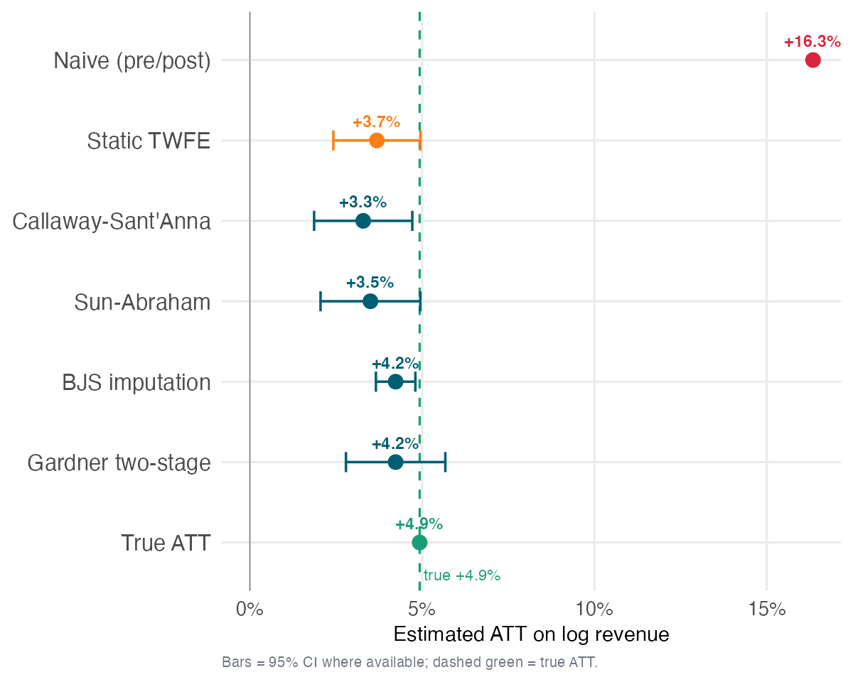
Four estimators converge — just below the truth

One tight band from four different algebras — the spread is weighting / efficiency, not disagreement. Convergence certifies the staggered-timing fix — not identification.

All four share the same additive-PT backbone, so they miss the truth together. That co-miss is the clue:

The gap motivates S11 & S12

An omitted regional-economy factor loads differently on treated vs control markets — a PT violation DiD’s additive model can’t see. S11 (synthetic control) & S12 (counterfactual imputation) are built to.

The credibility payoff and the session’s intellectually honest centerpiece, on one slide, placed here so it lands as convergence after all four estimators have been built rather than as a lone claim. First the convergence argument: four estimators resting on genuinely different algebra — CS’s group-time two-by-twos, SA’s saturated interaction-weighted regression, BJS’s efficient imputation, Gardner’s two-stage imputation — all land in the tight band plus 3.3 to 4.2 percent. That agreement is the real argument — but say precisely what it buys. The four differ in their AGGREGATION mechanics (how each dodges the forbidden comparisons of staggered timing), so their convergence certifies that the staggered-timing fix works: none is idiosyncratically broken by the timing problem. Read the two gaps differently. The roughly 0.9-percentage-point spread WITHIN the band (CS plus 3.3 up to BJS/Gardner plus 4.2) is a weighting-and-efficiency difference around one target — CS’s overall-weighting versus BJS’s multiple-pre-period efficiency — not a disagreement about the effect. What convergence does NOT certify is identification, because all four rest on the SAME additive unit-plus-time / parallel-trends backbone, so they can, and here do, miss TOGETHER. This is the key correction to the slippery “independent methods agree, so we’re right” move: agreement under a shared assumption cannot vouch for that assumption. Contrast static TWFE, which happens to sit near plus 3.7 percent but for the WRONG reason (forbidden comparisons dragging it down), so proximity there is luck, not credibility. Now the deliberate reversal — and this is the discipline of the slide — resist claiming victory. The cluster converges SYSTEMATICALLY BELOW the true plus 4.9 percent, not to it, and the gap is real and informative, not noise. Its source is an omitted REGIONAL-ECONOMY factor — a slow latent wave whole regions ride together, loaded differently by treated versus control markets — a mild parallel-trends violation the pre-test was underpowered to catch (Roth), and one DiD’s additive unit-plus-time model structurally cannot represent because the factor interacts unit and time. Be precise if a student asks WHICH factor: it is the regional wave, not the coffee seasonality. Seasonality is real in this DGP, but the common time effect absorbs its average, and what survives contributes almost nothing to the bias; the regional wave is the one that moves the estimate. Do NOT say the robust estimators recover the truth; say they earn a defensible band and hand you a clue. That clue is the course’s argument for what comes next: synthetic control (S11) matches pre-treatment trajectories and can absorb such a factor, and counterfactual imputation (S12) — re-reading BJS’s recipe with a flexible factor model — models it explicitly. This is why DiD is the beginning of Part V, not the end.

Conditioning on Covariates

When parallel trends needs a covariate

Sometimes raw parallel trends fails, but a conditional version holds — treated and control move in parallel within strata of covariates \(\mathbf{X}\). Conditioning switches on two assumptions raw DiD never needed:

(A.cpt) Conditional parallel trends

\(\mathbb{E}[\Delta Y(0)\mid D{=}1,\mathbf{X}] = \mathbb{E}[\Delta Y(0)\mid D{=}0,\mathbf{X}]\) — with \(\mathbf{X}\) not affected by treatment.

(A.cna) Conditionally no anticipation

No pre-launch effect within each \(\mathbf{X}\)-stratum — the treated and control paths coincide before \(g\) given \(\mathbf{X}\).

(A.pos) Overlap / positivity

Every treated \(\mathbf{X}\) has a control that shares it: \(0 < \Pr(D{=}1\mid\mathbf{X}) < 1\). Watch this one — on BeanBuzz it breaks.

Set up covariate adjustment as the natural next question in the estimation half. Unconditional parallel trends can fail while a conditional version holds — the treated and control markets need not move in parallel overall, only within cells of covariates X. That is (A.cpt), conditional parallel trends, with the crucial rider that X must not be affected by treatment (a pre-treatment / time-invariant characteristic). Two more assumptions switch on the moment you condition. (A.cna) conditionally-no-anticipation: within each X-stratum there is no treatment effect before launch g — the honest completion of the identification trio (it is what lets the pre-period differences identify the counterfactual trend). (A.pos) overlap/positivity: for every covariate profile among the treated there must be controls sharing it, so the propensity is strictly between 0 and 1. Flag A.pos hard now, because on BeanBuzz it is exactly this assumption that breaks — the rollout went to the biggest markets first, so conditioning on size makes “treated” almost perfectly predictable and overlap collapses. We watch it happen on the forest slide. A.pos lives only in the propensity-using estimators (IPW, DR); OR/TWFE/imputation carry no overlap requirement.

Which covariates actually confound a trend?

Two axes decide it: is the covariate fixed or moving, and is its effect on \(Y\) fixed or moving?

	effect on \(Y\) time-invariant	effect on \(Y\) time-varying
\(X_i\) fixed	harmless — level gap absorbed by \(\alpha_i\)	confounds — different levels × a changing effect
\(X_{it}\) moving	confounds iff groups evolve differently	confounds — differential evolution &/or changing effect

The catch: an additive control does nothing

A fixed \(X_i\) added additively is collinear with \(\alpha_i\) → silently dropped. It only adjusts through a time-varying channel — \(X_i\times t\), or a differenced-outcome model. Ask: does \(X\) move the trend, or just the level?

Selection alone is not confounding

A covariate can also predict who gets treated (\(X\to D\)) — but that alone does not bias DiD: differencing absorbs fixed levels, so DiD tolerates selection on time-invariant traits. It bites only if the selector also moves the trend (but conditioning on a strong selection driver can break overlap).

The taxonomy the current deck dropped and the old deck carried (old slides L381-405). Cross two axes: covariate type (time-invariant X_i vs time-varying X_it) × effect type (time-invariant vs time-varying). Read the four cells. Top-left: a fixed X with a fixed effect is a constant level difference — the unit FE alpha_i absorbs it, harmless. Top-right (a real confounder): X_i fixed but its EFFECT grows over time — the load-bearing AND rule: X_i confounds iff group means DIFFER and it has a time-VARYING effect (e.g. lot-size differs near the freeway AND outdoor space appreciates over the build window). Bottom row (X_it moving): confounds iff the groups’ covariate means evolve DIFFERENTLY, or they start different and evolve in parallel while the effect changes (an OR with a compound branch). Keep this distinct from cross-sectional confounding (mere X-treatment-outcome association) so students don’t import selection-on-observables reflexes.

Then the single most important econ point, entirely missing from both decks — the unit-FE ABSORPTION fact: in any within/FE regression a strictly time-invariant regressor is collinear with alpha_i and silently dropped. So a time-invariant covariate entered ADDITIVELY does nothing — it is exactly what plain DiD already differences out. It can only bite through a time-varying channel: X_i x t (TWFE/SA/imputation) or CS’s differenced-outcome nuisances (differencing removes alpha_i, so the baseline X survives). This is why every per-estimator entry two slides on uses X x t, not +X. The recurring test — “does X move the trend or just the level?” — decides whether a covariate earns a place at all. On BeanBuzz all four adjustment covariates (market_size, urban_share, seats, competitor_density) are strictly time-invariant, so this absorption fact is not academic — it dictates how every estimator must enter them.

Then the second callout, which pre-empts the natural student question “but what about a covariate that drives selection INTO treatment?” The correction to make firmly: selection is NOT a separate confounding channel. A covariate that only predicts who gets treated (X -> D) does not bias DiD by itself — differencing removes the unit fixed effect, so treated and control are allowed to differ arbitrarily in fixed levels and time-invariant traits. DiD is BUILT for selection on fixed characteristics (the old deck called the handled case “cross-sectional confounding” — what cross-sectional matching must control for but DiD gets for free). Selection bites ONLY when the selecting covariate ALSO moves the trend — i.e. it re-enters the 2x2 above (a time-varying effect / differential evolution -> conditional PT, A.cpt). So there is really ONE confounding question (does X move the trend?), plus two riders worth saying aloud: (1) because DiD tolerates pure level/selection, do NOT reflexively condition on a selection driver — a strong one you don’t need can only hurt; (2) the sharp irony — the STRONGER a covariate drives selection, the more conditioning on it BREAKS overlap/positivity (putting a near-deterministic selector in the propensity model pins e(X) at 0/1 and wrecks A.pos). Keep this GENERIC here — the BeanBuzz-specific slides that follow name the concrete selection driver and show the overlap break live, so do not pre-empt that reveal. One case conditioning canNOT fix, for completeness: selection on the transitory shock or the expected gain itself (Ashenfelter-dip-style, or selection on anticipated treatment effects) — that violates parallel trends directly and no covariate adjustment repairs it; it needs a different design.

Time-varying \(X\): pin it at pre-treatment — or model it

Most estimators treat every covariate as time-invariant — a moving \(X_{it}\) is fixed at its pre-launch value:

• Why: a post-launch \(X_{it}\) the app changed is a mediator — a bad control (next slide). Fixing it also cuts dimensionality.
• Cost: you no longer control a genuinely different evolution in \(X_{it}\) — that PT violation survives.

If \(X_{it}\) is exogenous to treatment (given its past): a doubly-robust estimator may use its post-treatment values, or you regression-impute the counterfactual \(X_{it}(0)\). (Caetano et al. 2024)

On BeanBuzz the four adjustment covariates are all time-invariant — this rung is the theory you’d need if they weren’t.

The “how do time-varying covariates enter” rung, mined from the old deck’s Handling-of-Confounding-Covariates slide (L407-420). The default convention across essentially all modern estimators: treat every covariate as time-invariant by fixing a time-varying X_it at its pre-treatment (base-period) value. Two reasons — it avoids conditioning on a post-treatment X the treatment itself moved (a mediator / bad control, next slide), and it slashes dimensionality. The cost is real: you then cannot control a covariate that genuinely evolves differently across groups independent of treatment, so that particular PT violation survives. The more-recent recommendations (Caetano et al. 2024): if X_it is EXOGENOUS to treatment conditional on its past, a doubly-robust estimator may legitimately use its post-treatment values; or use a regression-imputation approach that predicts the counterfactual post-treatment covariate value X_it(0). This is the one licensed case for conditioning on a post-treatment covariate, and it is DR-family only — pure OR/IPW do not get the licence. Honest caveat for this class: all four BeanBuzz adjustment covariates are strictly time-invariant, so this rung is off-data theory — the panel does carry time-varying covariates (footfall, temperature, marketing spend) you could use to demonstrate it, but none is a confounder of the launch. Verified: did::att_gt on a BALANCED panel silently coerces a time-varying X to its base-period value anyway, so even passing one usually buys no genuine time-varying adjustment.

Which covariates? The bad-control trap

More covariates is not safer. A covariate the treatment affects is a bad control:

• Mediators / post-treatment covariates — conditioning on them subtracts part of the effect (over-control). (Caetano et al. 2024)
• The “kitchen-sink” TWFE — throwing in every \(X_{it}\) — can bias the estimate, not clean it.

Rule: condition only on pre-treatment characteristics that could confound the trend — never on a consequence of the app. (Assignment V makes you make exactly this call.)

Close the “which covariates” question with the judgment that decides whether covariate adjustment helps or hurts — the same good-control/bad-control logic from the confounding sessions (S02, S06), now in DiD. The danger is not too few covariates but the wrong ones: a covariate the treatment itself affects is a bad control. Condition on a mediator or any post-treatment covariate and you subtract part of the very effect you are measuring (over-control bias). The “kitchen-sink” instinct — throw every available X_it into the TWFE — can actively bias the estimate rather than clean it (Caetano-Callaway). The mechanic for a treatment-affected time-varying X (fix at pre-launch, or drop) was the previous slide; here state the exclusion rule plainly: only condition on PRE-treatment characteristics that could plausibly confound the trend, never on a consequence of the app. Assignment V Step 5 hands students a covariate (staffed lanes) the treatment affects and grades whether they leave it out — so this slide is also their preparation. This slide now leads INTO the per-estimator machinery rather than closing the act.

Where \(X\) enters TWFE and Sun-Abraham

Both are one feols regression, so \(X\) enters as the same hand-written term — only the treatment block differs (\(\tau(D_i{\times}t)\) or i(rel,ref=-1) for TWFE, sunab(g,week) for Sun-Abraham). Pick the covariate × effect combination (Zeldow and Hatfield 2021):

covariate × effect	cov term	fixest
fixed \(X_i\) × time-varying effect	\(\delta\,(X_i\times t)\)	+ i(week, X)
moving \(X_{it}\) × fixed effect	\(\delta\,X_{it}\)	+ X
moving \(X_{it}\) × time-varying effect	\(\delta\,(X_{it}\times t)\)	+ i(week, X)

The covariate block is identical for the event study and for Sun-Abraham — only the treatment block beside it changes.

The shared price (Caetano-Callaway)

Homogeneous-in-\(X\), linear-in-\(X\), adjusts changes not levels. Difference: on TWFE it can’t fix the staggered-timing bias (decorates a biased estimator); on SA it rides an already-clean one. (Caetano et al. 2024)

The per-estimator ask for TWFE, reviving the old deck’s three Zeldow-Hatfield specs (old L498-513) that the current deck dropped. Covariate-TWFE is the one family where you EXPLICITLY choose the (covariate type) x (effect type) combination, because you hand-write the term — there is no covariate argument. Walk the table: (i) a time-invariant X_i with a time-VARYING effect enters as delta(X_i x t), coded i(week, X) — this is the safe workhorse and exactly what the cache computes (urban_share x week, +3.5%); (ii) a time-varying X_it with a constant effect enters additively as delta X_it, coded + X; (iii) a time-varying X_it with a time-varying effect enters as delta(X_it x t). Note (i) and (iii) share the fixest idiom i(week, X); the difference is whether X itself moves. For the event study, interact the covariate with event-time, i(rel_time, X). Then the price, stated plainly (Caetano-Callaway): the additive-linear form bakes in a treatment effect homogeneous across values of X, outcome linear in X, and adjusts covariate CHANGES not levels; and — the point students miss — covariate-augmented TWFE does NOT touch the staggered-timing / negative-weighting bias. Adding X x t decorates a biased estimator; the forbidden-comparison problem is orthogonal to covariate adjustment. Use the imputation/DR estimators (next slide) that impute from clean untreated cells. SUN-ABRAHAM INTEGRATION (professor): because sunab() is just a fixest term, covariate-Sun-Abraham is the SAME feols regression as covariate-TWFE — the covariate block (the three specs and their fixest idioms) is identical; you only swap the treatment block (tau(D×t) / i(rel,ref=-1) -> sunab(g,week)). Verified this session: feols(log_rev ~ sunab(ft_sa,week) + i(week, urban_share) | sid+week) = +3.4%, the exact same +i(week,X) term as the covariate-TWFE +3.5% row. The Caetano caveats (homogeneous-in-X, linear-in-X, changes-not-levels) apply to BOTH; the only difference is that TWFE’s covariate decorates a still-biased estimator (covariates don’t touch the staggered-timing bias) whereas SA’s rides an already-de-biased one. One SA-specific nuance: the additive X sits OUTSIDE the sunab cohort×event-time saturation, so it imposes a single common X-slope across cohorts (a homogeneous-in-X conditioning weaker than CS’s per-(g,t) nuisance).

Callaway–Sant’Anna’s doubly-robust model on \(\Delta Y\)

C&S’s default (est_method="dr") puts \(X\) into two nuisance models on the change \(\Delta Y = Y_t - Y_{g-1}\) (\(\alpha_i\) differenced out) (Sant’Anna and Zhao 2020):

• Outcome \(\;\hat m_0(\mathbf X)=\mathbb E[\Delta Y\mid D{=}0,\mathbf X]\) — the control group’s expected change given \(\mathbf X\), imputed onto the treated.
• Propensity \(\;\hat e(\mathbf X)=\Pr(D{=}1\mid\mathbf X)\) — reweight controls to the treated’s \(\mathbf X\)-mix.

\[\widehat{\text{ATT}}(g,t)=\mathbb E_{D{=}1}\big[\Delta Y-\hat m_0(\mathbf X)\big]\;-\;\mathbb E_{D{=}0}\big[\hat w_e(\mathbf X)\,(\Delta Y-\hat m_0(\mathbf X))\big],\quad \hat w_e\propto\tfrac{\hat e}{1-\hat e}\]

covariate × effect	what C&S can model (the difference decides)
fixed \(X_i\) × time-varying effect	the target — \(X_i\) predicts the differential change
moving \(X_{it}\) × fixed effect	drops out unless groups’ \(X\) evolve differently (base-period \(X\) won’t catch it)
moving \(X_{it}\) × time-varying effect	needs period-specific \(X\) → base-period coercion on a balanced panel

Two chances to be right: consistent if either \(\hat m_0\) or \(\hat e\) is right. Neyman-orthogonal, so fit both nuisances with ML — S09’s AIPW score = Chang’s DML-DiD. (Chang 2020)

The adapted S09/DR slide (professor): retitled to Callaway-Sant’Anna, repositioned right after the TWFE+SA regression-family slide so the two detailed “how each estimator takes covariates” slides sit together at the front of the per-family covariate slides. Goal: fully specify the doubly-robust estimator so students SEE both nuisance models on the first-differenced outcome. Differencing ΔY = Y_t − Y_{g-1} removes the unit FE alpha_i (which is why a baseline time-invariant X survives here). (1) Outcome model m0(X) = E[ΔY | control, X] — the Heckman-Ichimura-Todd control-change regression, imputed onto each treated unit as its counterfactual change. (2) Propensity model e(X) = Pr(D=1 | X) — Abadie’s IPW, reweighting ONLY the controls to the treated X-distribution. Doubly robust = combine both in the Sant’Anna-Zhao AIPW moment: the residual (ΔY − m0(X)) averaged over the treated minus its propensity-reweighted average over the controls; consistent if EITHER model is right (two chances). Because the residual appears in both terms with the propensity weights, first-order errors in either nuisance cancel — that is Neyman-orthogonality, and it is what licenses fitting BOTH m0 and e with ML (random forests, gradient boosting) without first-order bias in the ATT — exactly Chang’s double/debiased DiD. Keep ML conceptual: the reported BeanBuzz menu stays CS/SA/BJS/Gardner, no separate DML number. This IS S09’s orthogonal AIPW score, now on differences rather than levels — students already know the score. est_method=“reg” uses only m0; “ipw” only e(X); “dr” (the default) uses both. The CS cohort aggregation = panel GATE point (“disaggregate before you aggregate”) can be mentioned here if time allows.

BJS / Gardner: covariates in the \(Y(0)\) imputation

Both fit \(Y(0)\) on the untreated cells — now with a covariate term — then predict onto the treated (fit white, predict grey) (Borusyak, Jaravel, and Spiess 2024; Gardner 2022):

\[\underbrace{Y_{it}(0)=\alpha_i+\gamma_t+\delta\,(X_i{\times}t)+\varepsilon_{it}}_{\text{fit on untreated cells (the first stage)}}\ \longrightarrow\ \hat Y_{it}(0),\qquad \hat\tau_{it}=Y_{it}-\hat Y_{it}(0)\]

• \(X\) enters the first_stage via the same three specs as TWFE/SA — \(X_i{\times}t\) · \(X_{it}\) · \(X_{it}{\times}t\). BJS = Gardner (identical entry; differ only in SE).
• No propensity → no overlap needed (unlike CS-IPW/DR); but OR-family, so not doubly robust.

You can even impute \(X(0)\)

A time-varying \(X_{it}\) the treatment moved is a bad control. Instead impute its counterfactual \(X_{it}(0)\) on the untreated cells (same recipe), then feed \(X_{it}(0)\) into the \(Y(0)\) model — imputation extends to the covariate. (Caetano et al. 2024)

The BJS/Gardner imputation-family covariate slide (professor), replacing the cross-estimator matrix — this completes the per-family trio (TWFE+SA regression, CS-DR, now imputation). The mechanism, identical in both packages: fit the untreated-cell Y(0) model WITH a covariate term — first_stage = ~ i(week, X) | sid + week in both did_imputation (BJS) and did2s (Gardner) — predict Y(0) onto the treated cells, average the realized-minus-imputed gaps. This is exactly the fit-white / predict-grey recipe from the imputation-intro slide, now with X in the white-fit model. Because the first stage is one feols model, the SAME three Zeldow specs apply (X_i×t / X_it / X_it×t): outcome-side estimators (TWFE, Sun-Abraham, BJS/Gardner) all take covariates as the identical feols term; only the treatment/estimation machinery differs. BJS = Gardner for covariate ENTRY (verified this session: both +4.15% with i(week,urban_share)); they differ only in the standard error (BJS efficient/analytic; Gardner two-stage). Key contrast with CS to state: no propensity model, so NO overlap/positivity requirement — an advantage on BeanBuzz, where conditioning on market_size breaks CS-DR’s overlap — but also NOT doubly robust: a misspecified Y(0) model biases them with no propensity backstop. Then the distinctive extension, the reason imputation is special: because these estimators already impute Y(0), they can also impute the COUNTERFACTUAL COVARIATE X(0). A time-varying X_it the treatment moved is a bad control — you must not condition on its observed post-treatment value; instead fit an untreated-cell model for X as well, predict X_it(0), and feed that counterfactual covariate into the Y(0) model (Caetano et al. regression-imputation). This is the one clean way to condition on a post-treatment covariate, and it falls naturally out of the imputation framework. Practical guardrail: never put the treatment variable in first_stage.

Seven candidate covariates: could confound vs. what they do

A covariate confounds only if it moves the trend and lines up with the biggest-first rollout — via one of the three specs. Here, most don’t:

Covariate	type	Would confound if… → which spec	In BeanBuzz it…
market_size	inv	big markets ride a size-scaled trend → (i) \(X_i{\times}t\)	drives the rollout — sets level & timing; conditioning breaks overlap
urban_share	inv	urban markets swing harder with seasonality → (i) \(X_i{\times}t\)	the real \(X{\times}t\) channel — loads the seasonal factor (\(+3.5\%\) row)
seats	inv	more seats bite harder as demand surges → (i) \(X_i{\times}t\)	decoy — not in revenue
competitor_density	inv	denser markets feel a growing competitive drag → (i) \(X_i{\times}t\)	decoy — not in revenue
footfall_index	var	an urban revival lifts treated footfall → (ii) \(X_{it}\)	decoy — a proxy of the common seasonality
temp_c	var	different climates × temp-sensitive demand → (ii) \(X_{it}\)	decoy — a common wave, absorbed by \(\gamma_t\)
mktg_spend	var	a size-scaled ad push over the window → (ii) \(X_{it}\)	bad control — jumps at launch (treatment-affected)

Only urban_share moves the trend (an observed seasonal loading); market_size drives selection; the rest are decoys — and mktg_spend is a consequence of the app.

The concrete BeanBuzz roster, motivating why we condition on the four we do and ignore the rest — one row per covariate, mechanism vs. reality. Ground truth from the generator (make_beanbuzz_panel.R): the untreated outcome is log_y0 = log_base(market_size) + secular_trend + L1·F1_t + L2·F2_t + eps. NOTATION — we index the two waves by SVD order throughout the course, i.e. by how strongly they actually show up in the de-meaned panel: F1 = the DOMINANT regional-economy wave (loaded by region), F2 = the WEAK coffee-seasonality wave (loaded by urban_share). Heads-up if you open the R script: its variable names are the other way round (the script’s F1_t is the seasonality cosine, F2_t the regional AR wave) — the script names them in the order they were written, we name them in the order they matter. Only three things touch the outcome — market_size (level), urban_share (loads the WEAK seasonality wave F2), and region (loads the DOMINANT regional-economy wave F1) — and region is NOT a student-visible covariate in the store panel, so the regional wave is a fully latent factor (it is the bulk of the residual gap S11/S12 chase; the seasonality wave contributes almost nothing to the bias).

Walk the seven. TIME-INVARIANT (X_i): (1) market_size — would confound a trend only with a size×time effect; here it sets the revenue LEVEL (absorbed by the unit FE) and DRIVES the biggest-first rollout (selection on level), so its real damage is breaking overlap when you condition on it, not trend confounding. (2) urban_share — the one genuine confounding channel: it loads the WEAK winter-seasonality wave F2 (the script writes that loading as L1 = 0.85 + 0.45·urban_share), a fixed covariate with a time-VARYING effect (Zeldow spec i), which is exactly why urban_share×t is the covariate-TWFE adjustment (+3.5%); note it is drawn INDEPENDENTLY of size, so it is roughly balanced across cohorts and its bias is mild. (3) seats and (4) competitor_density — pure decoys, they never enter log_y0; each is given a plausible could-confound story (capacity constraints on a demand surge; a differential competitor-entry wave) so students see the mechanism they’d have to argue. TIME-VARYING (X_it): (5) footfall_index = f(the seasonality cosine, store noise) — a noisy proxy of the COMMON seasonal factor (the WEAK wave F2), not market-loaded, not in revenue; could matter only if footfall evolved differentially (urban-revival story). (6) temp_c = a common seasonal cosine identical across all stores → absorbed entirely by the time FE γ_t; could matter only with differential climate exposure × temperature-sensitive demand — the observable cousin of the latent factor. (7) mktg_spend = 400·market_size + 250·app_live + noise — it RESPONDS to treatment (jumps at launch) but has no arrow into revenue, so it is the bad-control-shaped decoy; it would be a real confounder only under an exogenous, size-scaled ad push decided independently of the launch. Bottom line for students: enumerate candidates, argue the trend-moving mechanism for each, and most fall away — leaving urban_share (adjust via X×t), market_size (the selection driver you must NOT over-condition on), and a latent regional factor no observed X proxies.

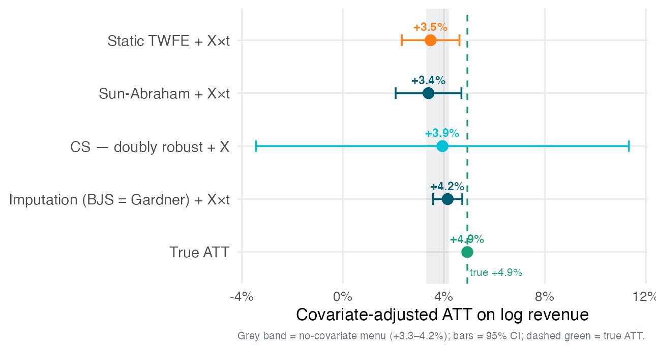
The covariate forest: \(X\) rescues none of them

Condition each estimator its own way — still the +3–4% band, below truth:

Covariates are not the fix

The band neither tightens nor reaches +4.9%; conditioning on size breaks overlap (C&S-DR’s CI explodes). The residual is a latent factor no \(X\) proxies → S11 / S12.

The closing forest, ask (c), built as a standalone read-only artifact (make_s10_cov_forest.R → covariate_forest.png; reads the cached twfe_x and dr rows, computes SA/BJS/Gardner+X fresh with analytic SEs, seeded bootstrap for the one CS-DR CI — never re-runs the locked cache). Each estimator enters covariates via its NATIVE mechanism, verified this session: static TWFE + urban_share x t = +3.5% (biased tier, shown for contrast); Sun-Abraham + urban_share x t = +3.4%; Callaway-Sant’Anna DOUBLY-ROBUST + all four covariates = +3.9% (the “focus on DR” row); combined BJS=Gardner imputation + urban_share x t = +4.2% (identical to the digit — same untreated-cell Y(0) model). The punchline: the covariate-adjusted band (+3.4 to 4.2%) is NO tighter and NO closer to the true +4.9% than the no-covariate robust menu (+3.3 to 4.2%, the grey band) — covariates buy model-dependence, not accuracy. Then the sharper point on the CS-DR row: conditioning on market_size (the biggest-first selection driver) pins the propensity at 0/1, throws 412 overlap-violation warnings, and blows the CS-DR confidence interval wide open (roughly -3% to +11%) — the doubly-robust estimator you’d reach for is exactly the one overlap wrecks. A consistency note for a sharp student: CS-DR conditions on all four covariates (its nuisance models handle them); the regression/imputation family conditions on urban_share x t only, because a full four-covariate x week imputation first stage over-fits (BJS/Gardner collapse to +2.3% with a tripled SE) — urban_share is the leading biggest-first trend-shifter, so it is the defensible single control. The residual gap is the latent time-varying REGIONAL factor that no observed X proxies — and note the sting: urban_share, the one covariate that genuinely moves the trend, loads the SEASONALITY wave, which contributes almost nothing to the bias. So the covariate you can observe corrects the wrong wave, and the wave that matters is invisible. Representing it needs the factor models of S11 (synthetic control) and S12 (counterfactual imputation), not more controls. This is why DiD is the beginning of Part V, not the end.

Parallel Trends

Parallel trends is untestable — we escalate

Our headline +3.29% (Callaway-Sant’Anna) rests entirely on one assumption we can never check directly.

The untestable core

Parallel trends concerns the treated markets’ revenue had they never launched — a path that unfolds after launch and is never observed. A flat pre-trend is circumstantial evidence, never proof.

Our only visual test — the flat pre-trend — has three blind spots:

• Low power — a slow drift the pre-test rarely catches
• Wrong window — pre-flatness says nothing about a divergence that opens only post-launch
• Conditioning bias — keeping a study only when pre-trends “pass” selects on noise

Three tools of accelerating rigor close the blind spots: (i) the pre-trend eyeball (what we repair) → (ii) pretrends power quantifies low power (Roth 2022) → (iii) HonestDiD answers wrong-window + conditioning, subsuming the pre-test (Rambachan and Roth 2023).

This slide is the whole section in miniature — install it deliberately. Open by cashing the bridge: everything downstream, the +3.29 percent we will quote to the CFO, is only as good as parallel trends, and parallel trends is not a fact we can look up — it is a counterfactual we assert. Say the untestable-core line slowly: the estimand needs the treated markets’ no-app revenue path AFTER launch, and that path is by definition never in the data; the pre-period leads only interrogate the observed pre-window. So a flat pre-trend is circumstantial evidence, not proof — say that once, here, and never repeat it. Now the organizing move for the rest of the deck: the thing everyone does, eyeball a flat pre-trend, is a binary visual test (approach i), and it has exactly three blind spots. Low power — the pre-test is a weak instrument for slow drifts. Wrong window — even a perfect pre-test only certifies the pre-period; a divergence that opens at launch is untouched. Conditioning bias — Roth 2022’s ‘pretest with caution’: keeping only studies whose pre-trends passed selects on noise and distorts the estimate. Then the escalation, which is the argument: the flat pre-trend is the test we are REPAIRING, not one of the fixes. Two accelerating tools close its blind spots. Pretrends power (ii) QUANTIFIES the low-power blind spot — it tells us exactly how blind the eyeball is to a slow drift; it diagnoses, it does not by itself deliver robust inference. HonestDiD (iii) is the continuous sensitivity analysis that answers wrong-window and conditioning, and in fact subsumes the binary pre-test entirely. Rigor genuinely accelerates: pass/fail, then power-of-the-test, then full sensitivity. Tell them the next three slides are these tools in order. No figure here on purpose — this is the argument, not the evidence.

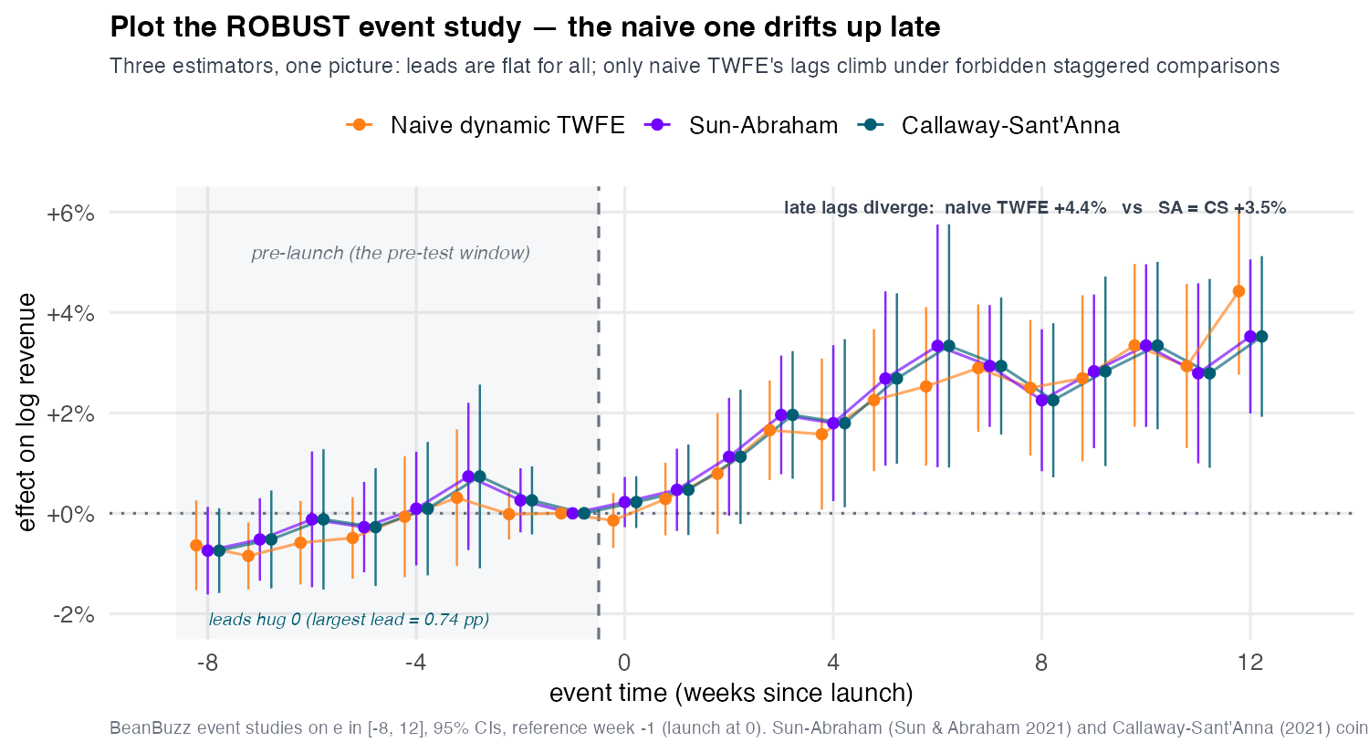
Trust the robust estimators, not the naive lags

• Leads (the pre-trend test) hug zero — largest 0.74 pp, none significant.
• Lags plateau at +2.95%; Sun-Abraham and CS coincide — only naive TWFE drifts up to +4.43%, forbidden-comparison contamination made visible.

Two recommendations

(1) What to read — the robust estimators, Callaway-Sant’Anna or Sun-Abraham (Sun and Abraham 2021); never the naive dynamic TWFE lags. (2) Base period — set base_period="universal" (hold \(e=-1\)): robust estimators build pre/post coefficients asymmetrically, so a default plot can fake a kink at zero (Roth 2024).

This is the visual test done right. Overlay the naive dynamic TWFE against the two robust estimators, Sun-Abraham and Callaway-Sant’Anna, on the window minus eight to plus twelve, each with 95 percent CIs and a common reference at week minus one. Read the leads first — remember leads are the pre-launch coefficients, our pre-trend test: all three hug zero, the largest is 0.74 pp at e = -8, and none is individually significant. By eye the treated and control markets moved in parallel before launch — the strongest circumstantial evidence a referee will expect. Read the lags second — the post-launch effect: the robust estimators ramp to a matured plateau near +2.95 percent from event-week eight on. Now the honest detail the overlay exists to show: Sun-Abraham and CS are numerically identical here — SA is the regression-level de-contamination of the naive event study, and on this data it lands exactly on the CS aggregation, so the two plot as one line (the figure annotates ‘SA = CS’). Only the naive dynamic TWFE separates, drifting UP to +4.43 percent by week twelve — the forbidden-comparison contamination from earlier in the deck, now visible: later naive lags borrow already-treated cohorts as controls. So recommendation one: read and trust the robust path, never the naive lags. Recommendation two, from Roth 2024: recent robust estimators construct pre- and post-coefficients against different references, which can manufacture a mechanical kink at event-time zero even with no effect and no pre-trend; hold a single universal base period — e = -1, common to every lead and lag, zero by construction — so a flat pre-period reads as genuinely flat, not as an artifact. Close on the handoff: flat leads are reassuring but not dispositive, and their three blind spots are exactly what approaches (ii) and (iii) now close.

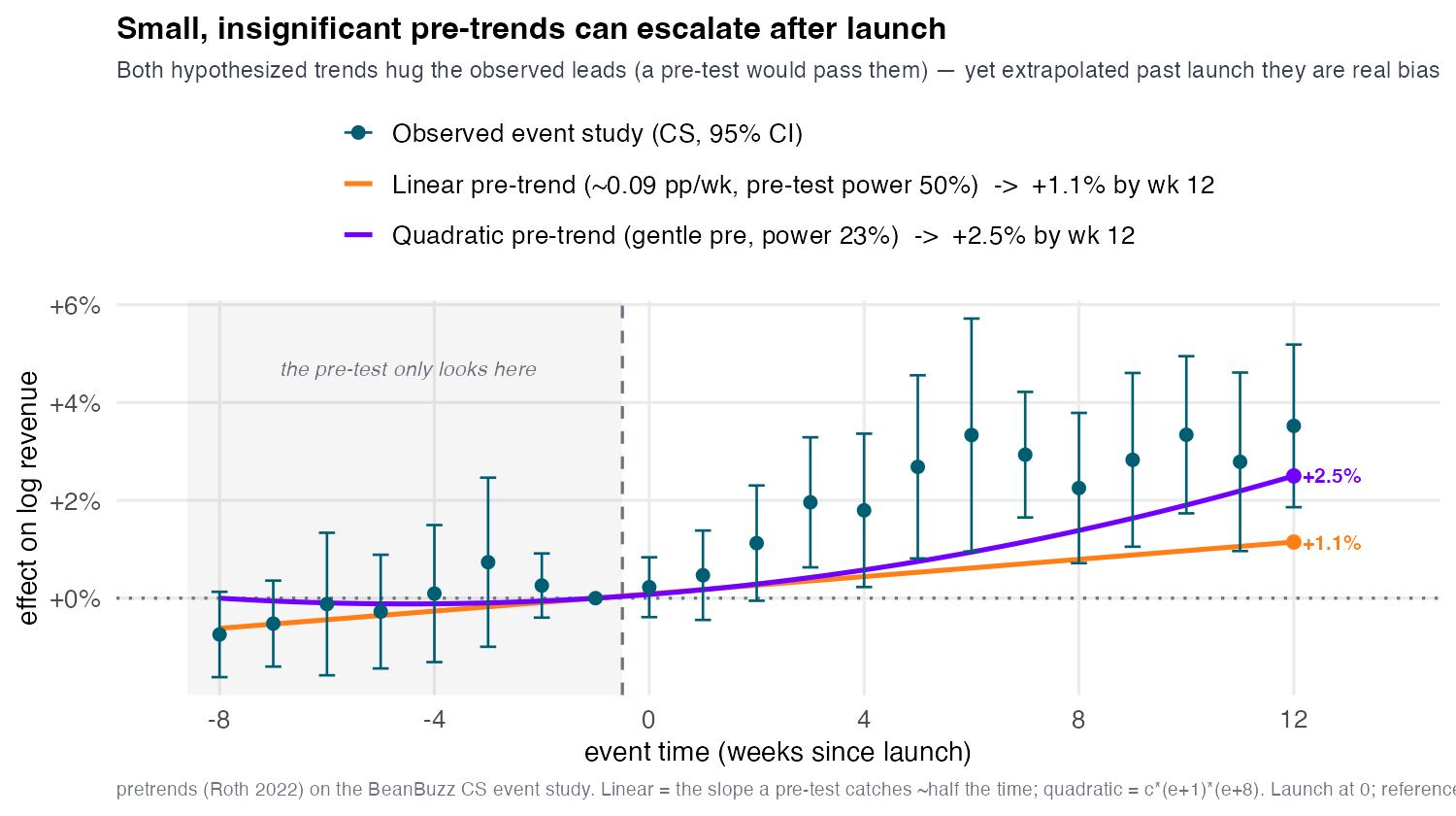
A biasing trend can hide in a flat pre-period

Blind spot (1) — low power, formalized. The pre-test jointly tests all leads = 0, so “passing” is only fail-to-reject, never confirm. slope_for_power() inverts it — the trend the test catches only a set fraction of the time; its bias is that trend extrapolated across the post window. (Roth 2022)

Both curves sit inside the leads’ error bars — a pre-test would pass them — yet grow after launch into real bias against a ~+3.5% effect:

• Linear 0.088 pp/week — caught only ~50% of the time → +1.15% by week 12.
• Quadratic (a convex path shaped to stay insignificant pre-launch) — caught only ~23% of the time → +2.5% by week 12.

Approach (ii): make the low-power blind spot concrete, and formalize why a pass is not proof. The pre-test is a JOINT test that all pre-treatment leads equal zero. Two things follow. First, its verdict is asymmetric: rejecting tells you there IS a pre-trend, but failing to reject only means you could not detect one — it never confirms parallel trends. Any drift small enough to hide inside the leads’ confidence intervals passes automatically. Second, Roth 2022 turns this into a power question and inverts it: instead of ‘did we reject?’, ask ‘what size trend would we catch, and how often?’ slope_for_power(0.5) returns the linear slope a pre-test rejects only half the time, and the bias such an undetected trend causes is that slope extrapolated across the whole post window. Now the figure. The petrol points are the observed CS event study we just trusted. The orange line is that linear trend — 0.088 pp per week, exactly slope_for_power at target power 0.5 (cache slope50 = 0.000882). Look at the shaded pre-window: it runs right through the leads’ confidence intervals, statistically indistinguishable from flat — that IS low power. Follow it past launch and it climbs to +1.15 percent by week twelve (0.000882 times 13) — real, systematic bias a flat pre-period gave us no way to rule out; against a roughly +3.5 percent effect that is a third of the result. The purple curve is a quadratic, and I want to be scrupulous: a raw quadratic in event time is symmetric and would blow up at the far leads, so the pre-test WOULD reject it — that would be a dishonest example. This curve is constructed as delta(e) = c(e+1)(e+8), anchored at the reference with its second root at the far lead, so by construction every pre-window value stays inside the observed leads’ CIs (verified programmatically); its true pre-test power is only 0.23 — even flatter in the pre-window, even harder to catch — yet it curves up faster after launch, to +2.5 percent. The honest pedagogical point: among violations the pre-test cannot distinguish from flat, a convex one does MORE post-period damage than a linear one. A point estimate needs a stress test, not a pre-test pass — which is approach (iii).

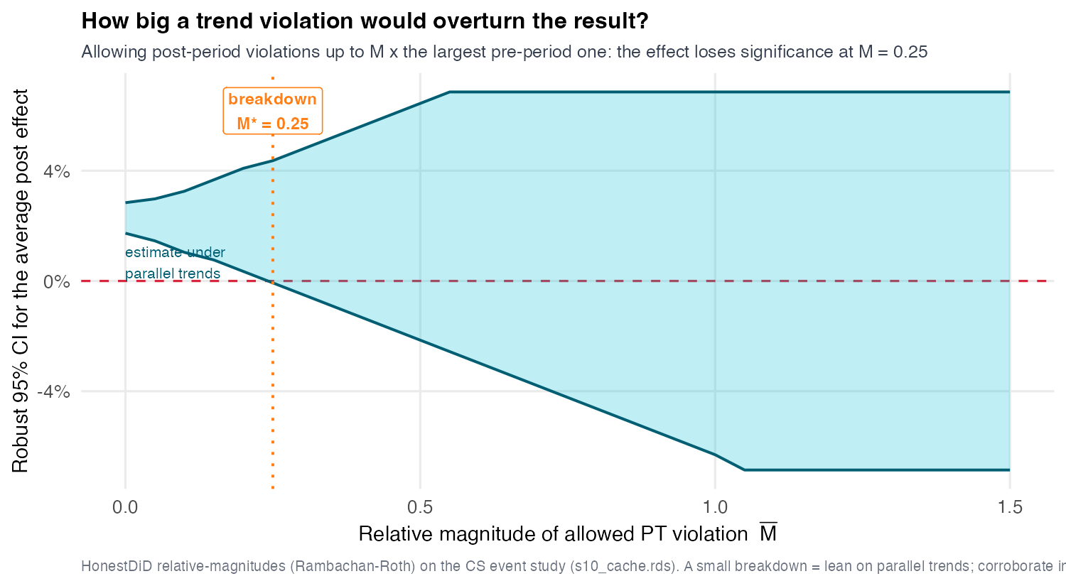
How big a violation before the effect breaks?

From pass/fail gate to yardstick

Stop asking “did the pre-trend pass?” Bound the unseen post-launch violation at \(\bar M \times\) the worst observed pre-period wobble; each \(\bar M\) yields an identified set and a confidence interval. The breakdown \(\bar M^{*}\) is the smallest \(\bar M\) whose CI first includes 0 (large → robust, small → fragile). This bounds the wrong-window violation the pre-test never saw, and replaces conditioning on a pass with the whole curve. (Rambachan and Roth 2023)

Name the object. The sweep stress-tests the +2.25% average post-launch effect (mean of the dynamic lags, weeks 0–12) — a more conservative aggregation than the +3.29% cohort-weighted headline. Robust CI runs [+1.73%, +2.84%] at \(\bar M=0\) → [−0.07%, +4.36%] at breakdown \(\bar M^{*} = 0.25\).

Approach (iii), the top of the ladder: replace the binary pre-test with a continuous sensitivity analysis (Rambachan and Roth 2023). The pre-trend stops being a pass/fail gate and becomes a yardstick — how big a post-launch violation, measured against the pre-period wobble, would overturn our conclusion? Relative magnitudes: M-bar bounds the unobserved post-launch violation as a MULTIPLE of the LARGEST observed pre-period violation — M-bar = 1 means ‘as bad as the worst divergence we actually saw before launch,’ M-bar = 0.25 ‘a quarter as bad.’ For each M-bar you get an identified set and a robust confidence interval; the breakdown value M-bar-star is the smallest M-bar whose CI first includes zero — large is robust, small is fragile. This directly attacks the two remaining blind spots: it bounds the wrong-window violation the pre-test never saw, and reporting the whole curve replaces conditioning on a single pre-test pass. A technical note for the curious, kept off-slide: the intervals plotted are the conditional least-favorable (C-LF) intervals, which invert the Andrews-Roth-Pakes moment-inequality tests; the fixed-length CI is the optimal interval under a different, smoothness restriction, not the relative-magnitudes sweep shown here — so do not conflate them. Now the honesty gate — say the object correctly. HonestDiD operates on the event-study coefficient vector, so its natural object is the AVERAGE of the dynamic post coefficients: +2.25 percent (cache dyn_overall = honest target_effect = 0.0225), the flat mean over weeks 0 to 12. That is a DIFFERENT aggregation than the +3.29 percent group-overall headline, which weights cohort ATTs over the full window; the +2.25 is dragged below the +2.95 percent matured plateau by the small early-ramp coefficients. It is also the more conservative object — it sits closer to zero, so it breaks sooner. Do NOT call the HonestDiD object +3.3 percent. Its original OLS CI is [+1.58%, +2.92%]; the robust menu the figure plots starts tighter, at the C-LF interval [+1.73%, +2.84%] at M-bar = 0, and widens to [-0.07%, +4.36%] at breakdown M-bar-star = 0.25, where the lower bound first crosses zero. Hand to the closer for the verdict.

BeanBuzz: clear under parallel trends, only moderately robust

Read \(\bar M^{*} =\) 0.25: a violation just a quarter as large as the worst pre-period wobble already overturns the average effect — the bias compounds over the horizon, so a drift invisible week-to-week accumulates across the plateau.

The honest verdict

The average post-launch effect is statistically CLEAR under parallel trends, but only MODERATELY robust to violations of it — not bulletproof. Because \(\bar M^{*} = 0.25 < 1\), we do not claim the effect survives violations as large as — let alone larger than — the worst we observed. The +3.29% headline leans on the same assumption; it is not separately shielded.

The Part V discipline — the same honesty as S09’s “is it real?”

A point estimate without a sensitivity analysis is not a finding. (Identify → impute → report a band + breakdown.)

Next (S11): corroborate with synthetic control — a method that does not lean on parallel trends.

The closer. Read the breakdown value plainly: M-bar-star = 0.25 means significance is lost once a post-period violation reaches just a QUARTER of the worst pre-period wobble. Why so small when the pre-trends looked flat? The bias on the average post effect COMPOUNDS over the post horizon — a drift invisible week-to-week accumulates across the plateau into something that matters; robustness to a full M-bar = 1 would require the effect to survive a post-violation as large as the worst pre-violation, and it does not. Deliver the professor-confirmed verdict and do NOT soften it: statistically CLEAR under parallel trends, but only MODERATELY robust to violations of it — not bulletproof. And explicitly refuse the overclaim: because M-bar-star = 0.25 is less than 1, we do NOT claim the effect survives violations as large as, let alone larger than, the worst we observed before launch — that would be false. Be precise about scope: it is the +2.25 percent average post-launch effect that is moderately robust; the +3.29 percent headline was never separately stress-tested and leans on the same parallel-trends assumption, so it is not independently shielded. Then the portable discipline, mirroring S09’s ‘is it real?’: a point estimate without a sensitivity analysis is not a finding — identify the assumption and the clean comparisons, impute Y(0), and report a band plus a breakdown, not a lone number. Close the deck on the S11 bridge: the honest next move is to corroborate with a method that does not lean on parallel trends at all — synthetic control, next session. This is the last content slide; only the References and the automatic Thank-you follow.

Baker, Andrew C., Brantly Callaway, Scott Cunningham, Andrew Goodman-Bacon, and Pedro H. C. Sant’Anna. 2025. “Difference-in-Differences: A Practitioner’s Guide.” arXiv Preprint arXiv:2503.13323.

Borusyak, Kirill, Xavier Jaravel, and Jann Spiess. 2024. “Revisiting Event-Study Designs: Robust and Efficient Estimation.” Review of Economic Studies 91 (6): 3253–85. https://doi.org/10.1093/restud/rdae007.

Caetano, Carolina, Brantly Callaway, Stroud Payne, and Hugo Sant’Anna Rodrigues. 2024. “Difference in Differences with Time-Varying Covariates.” https://doi.org/10.48550/arXiv.2202.02903.

Callaway, Brantly, and Pedro H. C. Sant’Anna. 2021. “Difference-in-Differences with Multiple Time Periods.” Journal of Econometrics 225 (2): 200–230. https://doi.org/10.1016/j.jeconom.2020.12.001.

Chaisemartin, Clément de, and Xavier D’Haultfœuille. 2020. “Two-Way Fixed Effects Estimators with Heterogeneous Treatment Effects.” American Economic Review 110 (9): 2964–96. https://doi.org/10.1257/aer.20181169.

Chang, Neng-Chieh. 2020. “Double/Debiased Machine Learning for Difference-in-Differences Models.” The Econometrics Journal 23 (2): 177–91. https://doi.org/10.1093/ectj/utaa001.

Gardner, John. 2022. “Two-Stage Differences in Differences.” https://doi.org/10.48550/arXiv.2207.05943.

Goodman-Bacon, Andrew. 2021. “Difference-in-Differences with Variation in Treatment Timing.” Journal of Econometrics 225 (2): 254–77. https://doi.org/10.1016/j.jeconom.2021.03.014.

Rambachan, Ashesh, and Jonathan Roth. 2023. “A More Credible Approach to Parallel Trends.” Review of Economic Studies 90 (5): 2555–91. https://doi.org/10.1093/restud/rdad018.

Roth, Jonathan. 2022. “Pretest with Caution: Event-Study Estimates After Testing for Parallel Trends.” American Economic Review: Insights 4 (3): 305–22. https://doi.org/10.1257/aeri.20210236.

———. 2024. “Interpreting Event-Studies from Recent Difference-in-Differences Methods.” arXiv Preprint arXiv:2401.12309.

Sant’Anna, Pedro H. C., and Jun Zhao. 2020. “Doubly Robust Difference-in-Differences Estimators.” Journal of Econometrics 219 (1): 101–22. https://doi.org/10.1016/j.jeconom.2020.06.003.

Sun, Liyang, and Sarah Abraham. 2021. “Estimating Dynamic Treatment Effects in Event Studies with Heterogeneous Treatment Effects.” Journal of Econometrics 225 (2): 175–99. https://doi.org/10.1016/j.jeconom.2020.09.006.

Zeldow, Bret, and Laura A. Hatfield. 2021. “Confounding and Regression Adjustment in Difference-in-Differences Studies.” Health Services Research 56 (5): 932–41. https://doi.org/10.1111/1475-6773.13666.

Thank you for your attention!
	www.startupengineer.io/team/ihl/ christoph-ihl christophihl