library(readr); library(dplyr); library(ranger); library(estimatr)
set.seed(7)
df <- read_csv(here::here("materials/data/shopsphere_promo.csv"), show_col_types = FALSE)
Xdf <- df |> select(recency, frequency, monetary, tenure, age,
                    channel, email_opens, loyalty_member)
Y <- df$profit_30d; D <- df$coupon; n <- nrow(df); K <- 5

# (a) 5-fold cross-fit mu1 = E[Y|X,D=1], mu0 = E[Y|X,D=0], e = E[D|X] with ranger
fold <- sample(rep(1:K, length.out = n))
mu1 <- mu0 <- ehat <- numeric(n)
for (k in 1:K) {
  tr <- fold != k; te <- fold == k
  # ___ YOUR CODE: fit a ranger() on the treated-train rows (Xdf[tr & D==1, ], Y[tr & D==1]) -> mu1[te]; same for mu0 on the D==0 rows
  # ___ YOUR CODE: fit a ranger() of D[tr] on Xdf[tr, ] for the propensity; ehat[te] <- its predictions clipped to [0.02, 0.98]
}

# (b) assemble the AIPW score and confirm its mean = the ATE (~1.5)
# ___ YOUR CODE: psi <- (mu1 - mu0) + D*(Y - mu1)/ehat - (1 - D)*(Y - mu0)/(1 - ehat)
# ___ YOUR CODE: mean(psi)   # AIPW ATE

# (c) regress psi on the frequency band -> GATE per band, with SEs
band <- cut(df$frequency, breaks = c(-1, 1, 3, 6, Inf), labels = c("0-1","2-3","4-6","7+"))
# ___ YOUR CODE: lm_robust(psi ~ 0 + band) # each coefficient is a GATE with a valid SE13 Session 9: Treatment Effect Heterogeneity
13.1 Lecture Slides
13.2 Overview
Last week DML handed you one number — the ATE — with an honest interval. It told you whether the coupon works on average; it never told you for whom. This session stops averaging and lets the effect vary with the customer. The whole deck rides on a single move from S08: the per-unit AIPW score \(\psi_i\) we built to estimate the ATE is constructed so that \(\mathbb{E}[\psi \mid X = x] = \tau(x)\) — it is a noisy, unbiased label for the unseen conditional effect. Average it and you recover the ATE (S08); project it and you recover everything heterogeneous. That is the spine of the session: one score, four jobs. Project \(\psi\) on a pre-specified group \(\to\) the GATE; regress \(\psi\) on the full covariate vector \(\to\) the CATE \(\tau(x)\) (the DR-learner, the family that causal forests belong to); rank units by \(\hat\tau\) and integrate \(\to\) the RATE / TOC targeting curve; weight a classifier by \(\psi\) \(\to\) the policy \(\pi(X)\). The running example is ShopSphere, an online retailer whose marketing team emails a targeted coupon to lapsing and engaged customers — observational data, so the confounding that needed the S08 machinery is exactly what we cash in here. The de-confounded ATE estimate is a “meh” ≈€1.4–1.5 (the true ATE is €1.69), but the per-customer effect ranges from −€6.5 to +€20.8: the coupon reactivates persuadable lapsers and cannibalizes margin on loyal regulars. Estimation is the easy half; the hard half is earning belief in the estimate, because a flexible learner draws a wiggly \(\hat\tau(x)\) even from pure noise. So we estimate, then validate (is it real? is it worth it?), then act (ship an auditable rule).
Key takeaways
- The average lies; the score doesn’t. The ATE is \(\tau(x)\) collapsed to a point — heterogeneity needs no new identification, only the S08 unconfoundedness, not yet averaged. The AIPW score \(\psi_i\) with \(\mathbb{E}[\psi\mid X]=\tau(x)\) is the one object that powers the entire session.
- One score, four jobs. Average \(\psi\) \(\to\) ATE; group it \(\to\) GATE (with honest CIs, for free); regress it on \(X\) \(\to\) \(\tau(x)\); rank it \(\to\) RATE; weight a classifier by it \(\to\) policy. Every method today is “regress / rank / weight the score.”
- Predicting \(Y\) well is not estimating \(\tau\) well. S- and T-learners minimize outcome MSE, but \(\tau\) is a difference of two surfaces (the MCE decomposition). The methods that work — causal forests, R-learner, DR-learner — target \(\tau\) directly through an orthogonal score. Heterogeneity estimation is DML refusing to take the final average.
- Validate before you believe; ship a rule, not a curve. A flexible learner always returns a wiggle, so clear three gates — BLP (real?), RATE (worth it?), CLAN (sensible?) — before acting. The deliverable is a policy \(\pi(X)\), learned as weighted classification on \(\psi\); on ShopSphere a two-question policy tree beat treating everyone by +€1.24 / customer.
13.3 Lecture Notes
13.3.1 Heterogeneity is a harder estimation problem, not a harder identification one
13.3.1.1 The managerial question the ATE cannot answer
S08 closed with an average effect for the coupon and an honest \(\sqrt{n}\) confidence interval. That is the right answer to “does the coupon work on average?” — but a marketing director rarely asks it. The operational questions are: who responds, and by how much? Is the variation real, or did a flexible model invent it? And given the answer, whom do we actually treat? Three verbs organize the whole session — understand (\(\tau(x)\)), validate (is it signal?), act (\(\pi(X)\)). The conceptual move that unifies them is small and exact: S08 averaged the per-unit score into the ATE; S09 projects the same score on covariates. Stop averaging the score; start projecting it on \(X\).
13.3.1.2 The object we want: the conditional average treatment effect
The central estimand is the conditional average treatment effect (CATE) — the expected effect among customers who look like \(x\):
\[\tau(x) \;=\; \mathbb{E}\!\left[\,Y(1) - Y(0) \;\middle|\; X = x\,\right].\]
It is the same potential-outcomes contrast as the ATE, conditioned on \(X\) rather than marginalized over it. Three estimands sit on one ladder of granularity:
- ATE \(=\mathbb{E}[\tau(X)]\) — one number for the whole population (S08).
- CATE / IATE \(=\tau(x)\) — a function of the customer; the most personalized object, “individualized” though still an expectation over residual heterogeneity at \(x\).
- GATE \(=\mathbb{E}[\tau(X)\mid G]\) — the effect for a named, usually low-dimensional group \(G\) (a coarsening of \(\tau(x)\)).
The point students must leave with: \(\text{ATE} = \mathbb{E}[\tau(X)]\), so the ATE is not a different object — it is \(\tau(x)\) integrated. Heterogeneity is simply what you see before you take that final average.
13.3.1.3 Heterogeneity needs no new identification
A natural worry is that asking a harder question — a whole function instead of one number — must cost more assumptions. It does not. Any target parameter is a conditioning of the individual effect on some function \(f(X)\), and by the law of iterated expectations, with \(G = f(X)\) a function of the covariates,
\[ \mathbb{E}\big[Y(1)-Y(0) \,\big|\, f(X) = f(x)\big] = \mathbb{E}\Big[\,\underbrace{\mathbb{E}\big[Y(1)-Y(0) \mid X = x\big]}_{=\,\tau(x)} \,\Big|\, f(X) = f(x)\Big]. \]
If unconfoundedness \(\{Y(1),Y(0)\}\perp D \mid X\) identifies the outer average — the ATE — it already identifies the inner effect \(\tau(x)\), because that conditional contrast is \(\tau(x)\). Every aggregation with respect to a function \(f(X)\) — GATE, ATE, or a sorted group — is then identified too.
13.3.1.4 Two roles for a covariate: confounder versus effect-modifier
A variable in \(X\) can play two logically independent roles. A confounder \(C\) affects both \(D\) and \(Y\); ignore it and the effect is biased — you must adjust (the identification job of S06–S08). An effect-modifier \(H\) changes the magnitude of \(\tau(x)\); ignore it and the ATE is still unbiased, you simply miss the heterogeneity (the description job of today). A variable can be both, either, or neither. On ShopSphere frequency is both: it drives who gets a coupon (the firm targets by frequency) and how much the coupon helps. The discipline: you condition on \(C\) to remove bias; you let \(\tau\) vary with \(H\) to describe variation. Different jobs, often the same columns.
13.3.1.5 IATE or GATE? A bias–variance choice
How finely should we resolve the effect? Going to the individual level minimizes bias (you condition on everything) but maximizes variance — almost no data sit at any single \(x\), so individual estimates are noisy and hard to trust one at a time. Coarsening to a handful of groups injects bias (you average over within-group heterogeneity) but slashes variance and buys honest standard errors. The practical resolution is a division of labour that recurs all session: report GATEs (stable, interpretable, defensible CIs) and use the continuous \(\tau(x)\) as the engine that ranks and targets — even when no single \(\hat\tau(x)\) is individually precise. You do not need each point estimate to be precise for the ranking to be useful, which is exactly what validation and policy learning exploit.
13.3.1.6 The score whose conditional expectation is the effect
Recall the S08 AIPW pseudo-outcome — the per-unit doubly-robust signal built from cross-fitted nuisances \(\hat\mu_1, \hat\mu_0, \hat e\):
\[ \psi_i = \underbrace{\big[\hat\mu_1(X_i) - \hat\mu_0(X_i)\big]}_{\text{direct (outcome regression)}} + \underbrace{\frac{D_i\,(Y_i-\hat\mu_1(X_i))}{\hat e(X_i)} - \frac{(1-D_i)(Y_i-\hat\mu_0(X_i))}{1-\hat e(X_i)}}_{\text{bias correction (propensity-weighted residual)}}. \]
Its defining property — the spine of the whole session — is that its conditional expectation given \(X\) equals the conditional effect:
\[\boxed{\;\mathbb{E}\big[\psi \mid X = x\big] \;=\; \tau(x)\;}\]
So \(\psi_i\) is a noisy but unbiased label for the latent, unobservable \(\tau(X_i)\): we can never see \(Y(1)-Y(0)\) for any single individual, yet \(\psi_i\) is a valid stand-in in conditional expectation. That single identity licenses everything that follows.
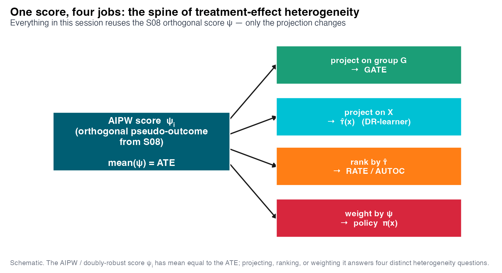
The roadmap is the spine in motion (Figure 13.1). Understand: estimate \(\tau(x)\) — first the coarse, reportable GATE, then forests and meta-learners for the continuous engine. Validate: a flexible learner will always hand you a wiggly \(\hat\tau(x)\), even from pure noise, so we test whether the variation is real (BLP) and worth acting on (RATE/TOC). Act: turn a validated \(\tau(x)\) into a deployable rule \(\pi(X)\). Estimation is easy; earning belief in the estimate is the work.
13.3.1.7 ShopSphere: the average effect is a trap
The running example is ShopSphere, an online retailer. The marketing team emails a targeted 15%-off coupon (\(D\)) and measures 30-day profit (\(Y = \texttt{profit\_30d}\), €). The covariates \(X\) are RFM-style: recency, frequency, monetary, tenure, age, channel, email_opens, loyalty_member. The data are observational: the firm already targets coupons at lapsing and highly-engaged customers, so \(D\) is confounded by the same covariates that drive profit. A naive treated-minus-control difference says the coupon destroys profit at −€1.38 — but coupon recipients are systematically lapsing customers who would have spent less anyway. The sign is confounded; this is precisely the Simpson-style reversal that needed the S08 machinery.
Run the S08 AIPW estimator with cross-fitted nuisances and the sign flips. The naive difference (−1.38) and the de-confounded AIPW estimate (R 1.40 / Python 1.52, CI covering the true ATE of 1.69) disagree in sign; a linear OLS with controls lands at 1.65, close but parametric. So the coupon adds about €1.4–1.5 on average — “meh.” A blanket campaign barely breaks even. But that average is the meaningless midpoint of a distribution that, as we will see, ranges from strongly negative to strongly positive. The average hides the action.
13.3.2 Report the group effect: GATE from the score
13.3.2.1 Three ways to get a group effect, only one of which de-confounds first
The simplest heterogeneity analysis splits customers into pre-specified, policy-relevant groups (frequency bands, channels, loyalty tiers) and estimates the effect within each. There are three classic strategies. (1) Stratify — rerun the full analysis in each subgroup; honest but data-hungry and high-variance for small cells. (2) An OLS interaction — fit \(Y = \alpha + \tau D + \gamma H + \delta(D\times H) + \varepsilon\) and read \(\delta\) as “how the effect varies with \(H\)”; tempting, but it inherits the confounding pathologies of the main effect, and the controls enter linearly. (3) DML on the AIPW score — regress the de-confounded score \(\psi\) on group dummies. Two discipline rules govern any of them: keep the groups coarse (few cells, so each has data and valid inference) and pre-specify them before peeking at outcomes — subgroups chosen after looking at \(\hat\tau\) are how false discoveries are born.
13.3.2.2 GATE = regress the score on the group
The spine, second appearance. Because \(\psi\) already has the confounding removed — it was built from cross-fitted \(\hat\mu_1,\hat\mu_0,\hat e\) — its conditional mean is \(\tau(x)\). So the GATE for group \(g\) is just the group mean of the score:
\[\widehat{\text{GATE}}(g) \;=\; \frac{1}{n_g}\sum_{i \,\in\, g} \psi_i \;=\; \bar\psi_{\,g}.\]
Operationally, an OLS of \(\psi\) on group indicators returns each GATE as a coefficient — with a valid standard error. Equivalently, write the AIPW ATE as the constant in \(\psi_i = \alpha + \varepsilon_i\) (so \(\hat\alpha = \widehat{\text{ATE}}\)), then extend it with the heterogeneity variable: \(\psi_i = \alpha + \beta\,G_i + \varepsilon_i\). We are modelling the level of the effect, not the level of the outcome.
13.3.2.3 Why the inference is valid: a proof of the AIPW–GATE identity
The validity rests on the spine identity \(\mathbb{E}[\psi \mid G = g] = \tau(g)\), proved by iterated expectations. Write the AIPW score at the true nuisances and condition on the group:
\[ \begin{aligned} \mathbb{E}\!\left[\psi_i \mid G_i = g\right] &= \mathbb{E}\!\left[ \mu_1(X_i) + \tfrac{D_i(Y_i - \mu_1(X_i))}{e(X_i)} - \mu_0(X_i) - \tfrac{(1-D_i)(Y_i - \mu_0(X_i))}{1 - e(X_i)} \;\middle|\; G_i = g \right] \\[4pt] &\overset{\text{LIE}}{=} \mathbb{E}\!\left[ \underbrace{\mathbb{E}\!\left[\mu_1(X_i) + \tfrac{D_i(Y_i - \mu_1(X_i))}{e(X_i)} \,\middle|\, X_i\right]}_{\text{AIPW for }\mathbb{E}[Y(1)\mid X]} - \underbrace{\mathbb{E}\!\left[\mu_0(X_i) + \tfrac{(1-D_i)(Y_i - \mu_0(X_i))}{1 - e(X_i)} \,\middle|\, X_i\right]}_{\text{AIPW for }\mathbb{E}[Y(0)\mid X]} \;\middle|\; G_i = g \right] \\[4pt] &= \mathbb{E}\!\left[ \mathbb{E}[Y(1)\mid X_i] - \mathbb{E}[Y(0)\mid X_i] \;\middle|\; G_i = g \right] \\[4pt] &\overset{\text{LIE}}{=} \mathbb{E}\!\left[Y(1) - Y(0) \mid G_i = g\right] \;=\; \tau(g). \end{aligned} \]
The inner conditional expectations are the per-arm AIPW signals, which equal the conditional average potential outcomes \(\mathbb{E}[Y(d)\mid X]\) under unconfoundedness and overlap; the outer LIE uses that \(G\) is a function of \(X\). Two facts then make the standard errors trustworthy. The score is orthogonal: small errors in \(\hat\mu_1,\hat\mu_0,\hat e\) do not contaminate \(\bar\psi_g\) to first order — the same Neyman orthogonality that made the S08 ATE valid. The groups are pre-specified and low-dimensional: a handful of fixed cells means ordinary OLS inference on \(\psi\) applies directly, with no post-selection penalty (Semenova and Chernozhukov 2021). Group-level heterogeneity therefore comes with honest confidence intervals essentially for free — which is exactly why GATEs are what you report to decision-makers. Computationally it costs only one extra OLS and no new nuisance parameters, and it is more flexible than the linear interaction because the confounding is absorbed by ML, not by a linear control. For a continuous modifier the same logic applies with the dummies replaced by a flexible basis — a series or kernel regression of \(\psi\) on the modifier (Semenova and Chernozhukov 2021).
13.3.2.4 The coupon helps the lapsed and hurts the loyal
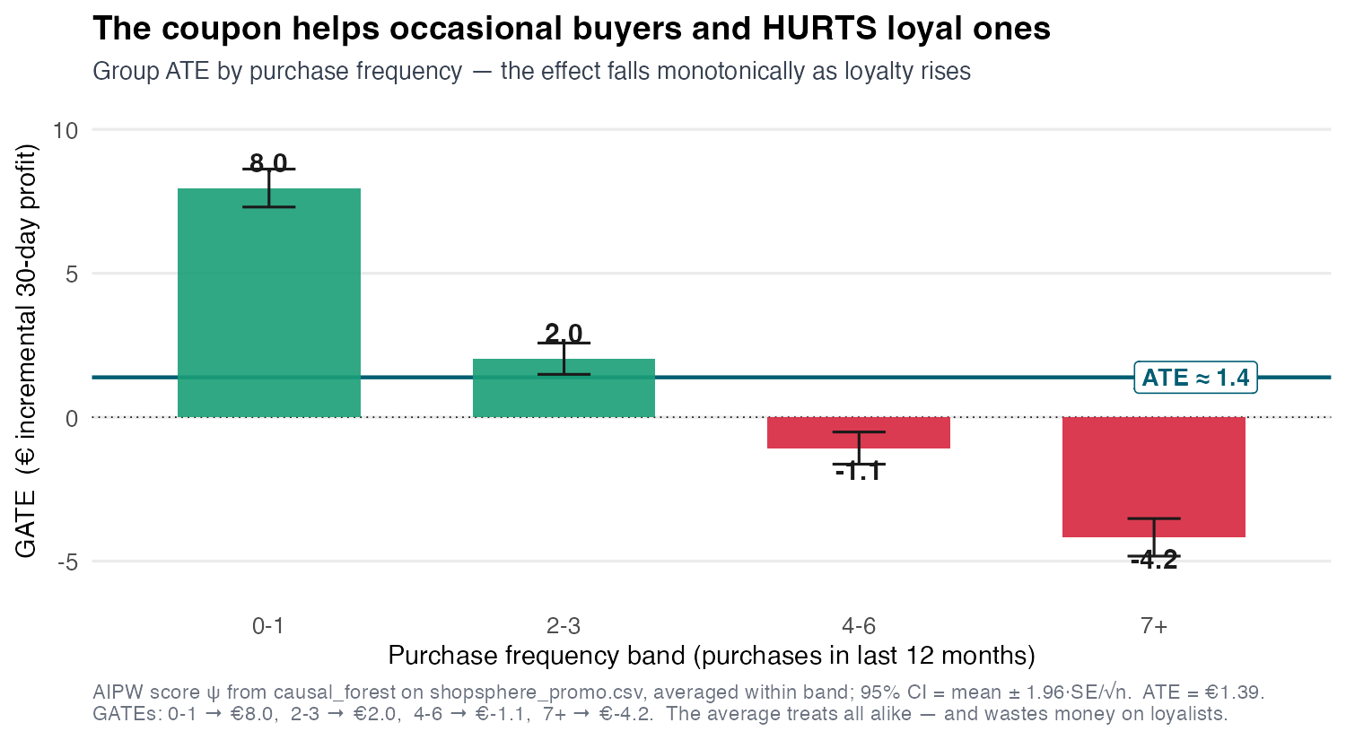
The GATE by frequency band (Figure 13.3) is the emotional core of the session. It moves monotonically from +€8.0 for lapsing customers (0–1 prior purchases) through near-zero to −€4.2 for the most loyal (7+ purchases). Business reading: coupons reactivate lapsing customers (the persuadables) but cannibalize margin on loyal customers who would have bought at full price (the “do-not-disturb” cell). This is the entire argument for targeting in one chart — and it is the coarse, reportable view. GATE is the communication layer you put in a slide deck for stakeholders; \(\tau(x)\) is the decision layer that drives the ranking and the targeting rule. You can report GATEs and still act on \(\tau(x)\) — complementary roles for the same object. But once the modifier is multivariate — frequency and recency and tenure — hand-picked bases break down, and we need a learner that finds the structure itself.
13.3.3 Estimating the engine: forests and meta-learners
13.3.3.1 The obvious idea, and why predicting \(Y\) well is not estimating \(\tau\) well
The meta-learner recipe builds \(\tau(x)\) out of off-the-shelf regressions. The S-learner (“single”) fits one model \(\hat\mu(D,X)\) with \(D\) as a feature and differences the two predictions, \(\hat\tau(x)=\hat\mu(1,x)-\hat\mu(0,x)\). The T-learner (“two”) fits \(\hat\mu_1\) on the treated and \(\hat\mu_0\) on the controls separately and subtracts. Both are intuitive and reuse any regressor — but both optimize the wrong objective. They minimize outcome prediction error (MSE on \(Y\)), while \(\tau(x)\) is a difference of two surfaces.
So the S-learner’s regularization can shrink the weak \(D\) signal toward zero — understating heterogeneity — while the T-learner’s two independently-tuned models differ in smoothness, so their difference inherits spurious structure (Curth and Schaar 2023). The cure is to target the causal quantity directly: split on effect heterogeneity (forests) or regress the orthogonal score (DR-learner).
13.3.3.2 Causal trees: split where the effect differs, then estimate honestly
A regression tree partitions \(X\) to make the outcome homogeneous within leaves. For a split of a parent node along variable \(j\) at point \(s\) into leaves \(L\) and \(R\), CART chooses \((j,s)\) to minimize the within-leaf sum of squared errors, which is equivalent to maximizing the sum of squared predictions \(\sum_i \hat{\ell}(X_i)^2\) — a reframing that matters because it needs only leaf means, not observed outcomes. A causal tree (Athey and Imbens 2016) changes the target: split to make the treatment effect differ across leaves, choosing \((j,s)\) to
\[ \max_{j,s}\;\Big[\, \textstyle\sum_{i: x_i \in L(j,s)} \hat\tau^2_{L(j,s)} \;+\; \sum_{i: x_i \in R(j,s)} \hat\tau^2_{R(j,s)} \,\Big], \]
where the leaf effect \(\hat\tau_{\text{leaf}}\) is the within-leaf treated-minus-control gap in experiments, or the within-leaf mean of the AIPW score under confounding. The danger is adaptive overfitting: choose the split and estimate the leaf effect from the same rows and you bias the effect toward the split — the search finds the rows where the effect looks biggest, so leaves look more extreme than they are.
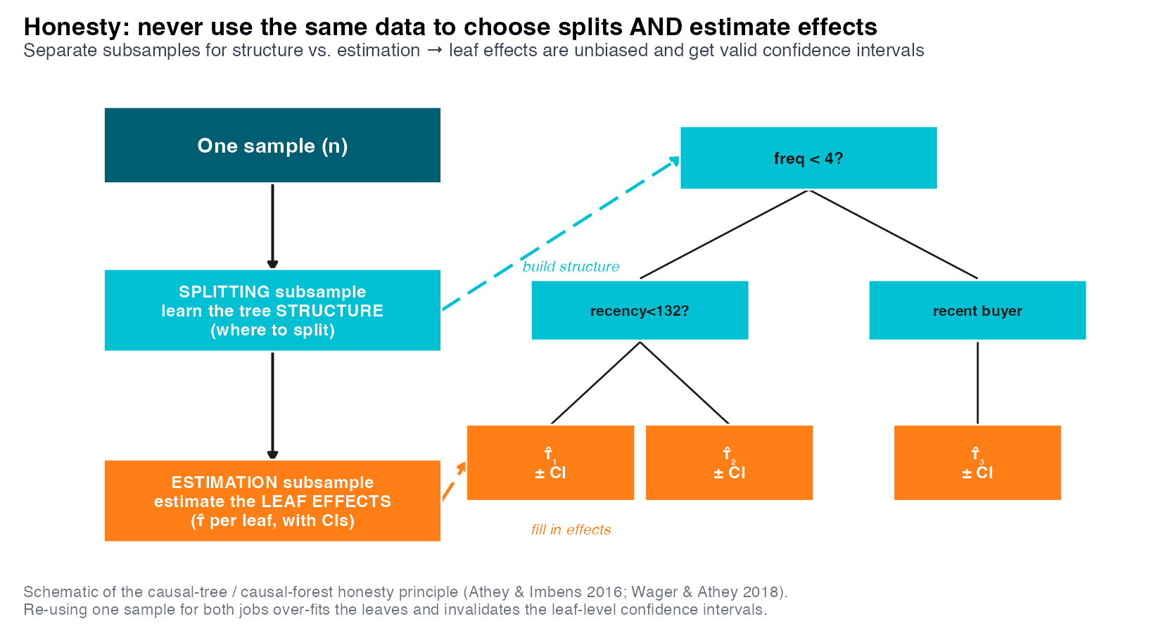
The fix is honest estimation (Athey and Imbens 2016) (Figure 13.4): use one subsample to choose the splits, a different subsample to estimate the leaf effects. The cost is statistical efficiency — half the data for structure, half for estimation — but the payoff is honest inference. This is the conceptual ancestor of cross-fitting: never let a unit be predicted by a model that was trained on it.
13.3.3.3 Causal forests: a learned similarity metric, and the local moment
A causal forest averages many honest causal trees, but it is more than an average (Wager and Athey 2018; Athey, Tibshirani, and Wager 2019). For a target point \(x\), each tree says which training units fall in \(x\)’s leaf — i.e. which units are “like \(x\).” Aggregating over trees yields smooth, data-driven adaptive weights \(\alpha_i(x)\): how much unit \(i\) looks like \(x\), with the forest deciding which covariates matter for similarity. The forest then estimates \(\hat\tau(x)\) by solving a locally-weighted version of the same partially-linear (residual-on-residual) moment we have used all along — units near \(x\) count more:
\[ \hat\tau^{\text{cf}}(x) = \arg\min_{\tilde\tau} \sum_{i=1}^N \alpha_i(x)\,\big[(Y_i - \hat{\ell}(X_i)) - \tilde\tau\,(D_i - \hat e(X_i))\big]^2, \]
with first-order condition (the local moment)
\[ \sum_i \alpha_i(x)\,\big[(Y_i - \hat{\ell}(X_i)) - \hat\tau^{\text{cf}}(x)\,(D_i - \hat e(X_i))\big]\,(D_i - \hat e(X_i)) = 0. \]
Here \(\hat{\ell}(X) = \mathbb{E}[Y\mid X]\) and \(\hat e(X) = \mathbb{E}[D\mid X]\) are the cross-fitted (or out-of-bag) nuisances from the first step. Read against the spine: DML set the unweighted average of the orthogonal score to zero to get the ATE; the causal forest sets a locally-weighted average to zero to get \(\tau(x)\). Same score family, same orthogonality (so the local estimate inherits robustness to nuisance error), just neighbourhood weights instead of uniform ones. In effect a forest is adaptive nearest-neighbour matching, where the distance metric is learned to track effect heterogeneity, not outcome level — which is exactly what fixes the S/T critique.
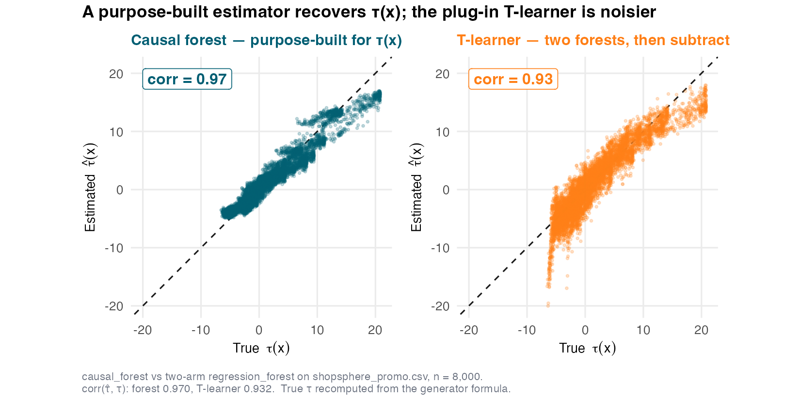
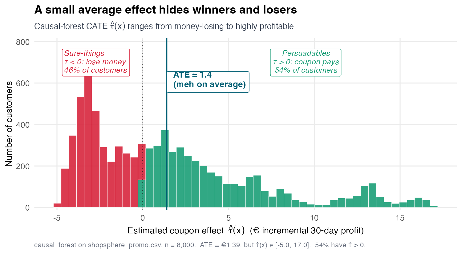
Because ShopSphere is simulated, we know the true \(\tau(x)\) and can plot estimate against truth (Figure 13.5). The causal forest hugs the 45° line at correlation 0.970 (Python 0.967); the T-learner is noisier at 0.932 (Python’s T-learner noisier still at 0.879, its DR-learner around 0.808 — an estimator-and-defaults gap we document in the lab rather than force-match). Across all customers the true effect \(\tau(x)\) ranges from about −€6.5 to +€20.8 (SD ≈ 5.7, 51.5% positive); the forest’s estimate \(\hat\tau(x)\) compresses that spread slightly to about −€5 to +€17 (SD ≈ 5.0, 54% positive), centred near the €1.4 forest ATE. The histogram of \(\hat\tau(x)\) (Figure 13.6) shows this estimated distribution directly. Either way the average was the tip of an iceberg — though remember a flexible learner can draw a wide histogram even from noise, so this is a hypothesis to be tested, not yet a finding.
13.3.3.4 A field guide to meta-learners: what each one regresses
The learners differ in what they regress. S and T regress the outcome \(Y\) and subtract predictions — indirect, the MCE critique applies. X, R, and DR target \(\tau\) itself.
The X-learner (Künzel et al. 2019) borrows strength under treatment imbalance (few treated, many controls — common in observational marketing). It (1) fits the T-learner’s \(\hat\mu_1, \hat\mu_0\); (2) imputes each unit’s effect using the other arm’s model — \(\hat D_{1,i} = Y_i - \hat\mu_0(X_i)\) for treated units, \(\hat D_{0,i} = \hat\mu_1(X_i) - Y_i\) for controls; (3) regresses the imputed effects on \(X\) within each arm to get \(\hat\tau_1, \hat\tau_0\), and blends by the propensity, \(\hat\tau(x) = \hat e(x)\,\hat\tau_0(x) + (1-\hat e(x))\,\hat\tau_1(x)\). The blend leans on the larger arm’s better-estimated model where data is thin. On ShopSphere treatment is balanced (50%), so the X-learner gains little here — but name the use case so students reach for it correctly. It is not doubly robust.
The R-learner (Nie and Wager 2021) targets \(\tau(x)\) through the Robinson partialling-out from S08, solved locally. Allowing the slope to vary with \(x\) in the partially linear model gives the outcome residual \(\tilde Y_i = Y_i - \hat{\ell}(X_i)\) equal to \(\tau(X_i)\) times the treatment residual \(\tilde D_i = D_i - \hat e(X_i)\), plus noise. The objective is
\[\hat\tau(\cdot) = \arg\min_{\tau}\ \sum_i \Big[(Y_i-\hat{\ell}(X_i)) - \tau(X_i)\,(D_i-\hat e(X_i))\Big]^2.\]
The DR-learner (Kennedy 2023) is the cleanest expression of the spine and our default. Condition the AIPW score on \(X\) — the same trick as the GATE, now with the full covariate vector:
\[\hat\tau(x) = \arg\min_{\tau}\ \sum_i\big(\psi_i - \tau(X_i)\big)^2 = \widehat{\mathbb{E}}\big[\psi \mid X = x\big], \qquad \mathbb{E}[\psi\mid X=x]=\tau(x).\]
Two stages: (1) cross-fit \(\hat\mu_1,\hat\mu_0,\hat e\) and build \(\psi_i\) (S08); (2) regress \(\psi_i\) on \(X\) with any flexible learner. Kennedy shows this is doubly robust and orthogonal, so the second-stage learner can be a black box without contaminating \(\tau(x)\) to first order. Concretely the cross-fitting rotates over folds: train \(\hat e\), train \(\hat\mu\), construct \(\psi\) and regress it on \(X\), then predict \(\hat\tau(x)\) — rotating so no unit’s score is built from a model that saw it. This is the third explicit reuse of \(\psi\), and it explains why the grf forest and the DR-learner agree so closely on ShopSphere: they fit essentially the same orthogonal target.
13.3.4 Is the heterogeneity real? Validation
13.3.4.1 A flexible learner always draws a wiggle
Fit a causal forest on data with zero true heterogeneity (\(\tau(x)\equiv\text{const}\)) and you still get a varying \(\hat\tau(x)\) — a wiggly histogram of pure noise. The estimate looks the same whether the heterogeneity is real or invented. Because we never observe a counterfactual, there is no classic out-of-sample test of the predicted effect against the realized one. The professional response is not to estimate and inspect individual CATEs but to derive summary statistics of their noisy distribution and test a joint hypothesis — that heterogeneity exists and the estimator detected at least part of it. Two distinct questions, two distinct tools: Is it real? (does \(\hat\tau\) carry signal about the truth — the BLP / calibration test) and Is it worth it? (would targeting by \(\hat\tau\) beat treating everyone — RATE / TOC).
13.3.4.2 The Best Linear Predictor: does \(\hat\tau\) predict the truth?
The Best Linear Predictor (BLP) of the true CATE by the estimated one is the (hypothetical) regression of \(\tau(X)\) on the demeaned prediction:
\[ (\beta_1, \beta_2) = \arg\min_{\tilde\beta_1, \tilde\beta_2}\ \mathbb{E}\Big[\big(\tau(X) - \tilde\beta_1 - \tilde\beta_2\,(\hat\tau(X) - \mathbb{E}[\hat\tau(X)])\big)^2\Big], \]
which (when it exists) gives, by the demeaning,
\[ \beta_1 = \mathbb{E}[\tau(X)] = \text{ATE}, \qquad \beta_2 = \frac{\operatorname{Cov}[\tau(X), \hat\tau(X)]}{\operatorname{Var}[\hat\tau(X)]}. \]
The decisive coefficient is \(\beta_2\). If \(\hat\tau = \tau\) then \(\beta_2 = 1\) (perfect calibration of the slope). If \(\beta_2 = 0\) the covariance is zero, which can happen for two reasons: either \(\tau(X)\) is constant (no heterogeneity to find) or \(\tau(X)\) varies but the estimator cannot find it (bad estimator or too little data). So testing \(H_0: \beta_2 = 0\) is a joint test of (i) the existence of heterogeneity and (ii) the estimator’s ability to detect it. In practice we operationalize the BLP via the spine — regress the orthogonal score \(\psi\) on the out-of-fold estimate:
\[\psi_i = \beta_1 + \beta_2\,\big(\hat\tau(X_i) - \overline{\hat\tau}\big) + \varepsilon_i,\]
where \(\beta_1\) calibrates the level (≈ ATE) and \(\beta_2\) calibrates the slope (when \(\hat\tau\) says “bigger,” is the effect actually bigger?) (Chernozhukov et al. 2018).
On ShopSphere the heterogeneity is unmistakably real — but read the two projections separately. The calibration test (test_calibration: the score \(\psi\) projected on the forest’s own prediction \(\hat\tau\)) returns a differential-prediction coefficient \(\beta_2 = \mathbf{1.08}\) with \(t = 36.6\) (slope ≈ 1, so the forest’s ordering matches the true ordering almost perfectly), rejecting \(H_0:\beta_2=0\) at \(p < 2\times10^{-16}\); the mean-forest calibration \(\beta_1 = 0.955\) confirms the level is right too. A separate call — best_linear_projection of the same score onto named covariates — then reads off the gradient: −€1.19 per purchase for frequency and −€0.028 per day for recency (both \(p < 2\times10^{-16}\)). The effect falls as customers buy more often, and is largest at moderate recency before fading once a customer has truly lapsed (Figure 13.8). These slopes corroborate Figure 13.3, but they are a gradient, not a dominance test: that frequency is the dominant modifier is the GATE bars’ verdict (and the standardized comparison — frequency ≈ −4.0 per SD versus recency’s −2.2), which the projection then confirms in direction. (Python’s manual \(\beta_2 = 1.30\), \(t = 43.8\) — same decisive conclusion, different scaling.)
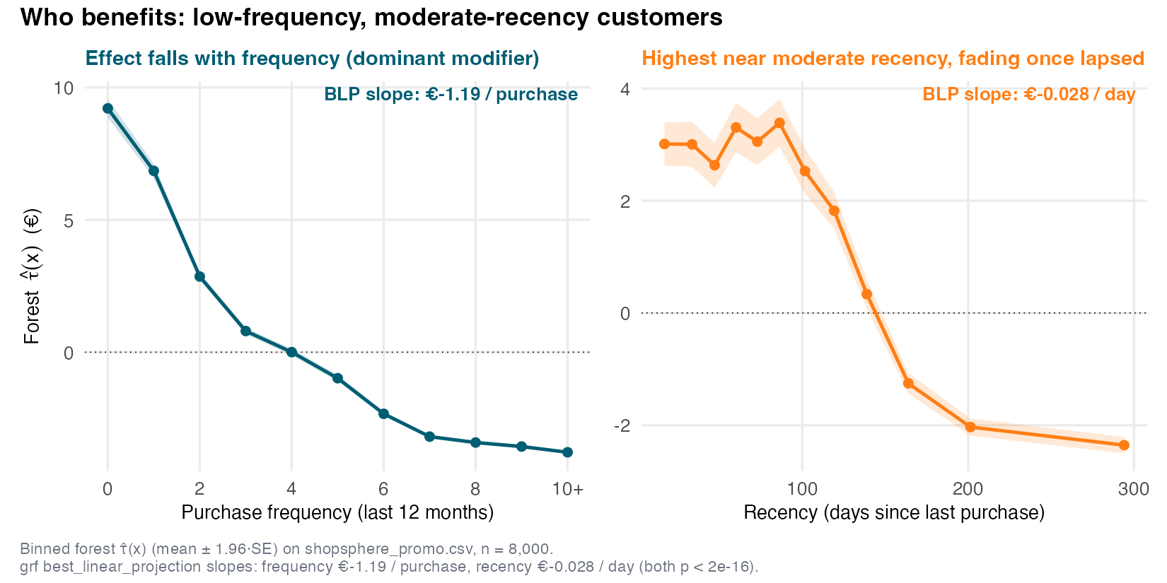
best_linear_projection slope overlaid. Left: the effect declines steadily with purchase frequency (BLP slope −€1.19 / purchase), from strongly positive for lapsing customers to negative for the most loyal. Right: it is highest near moderate recency (~70 days) and fades once a customer has truly lapsed (BLP slope −€0.028 / day). This is the continuous, multivariate generalization of the GATE-by-band view in Figure 13.3 — the BLP slopes turn the picture into two defensible numbers.
13.3.4.3 Is it worth it? RATE, the TOC curve, and QINI
Real heterogeneity is necessary but not sufficient — we need to know targeting pays. The Rank-weighted Average Treatment Effect (RATE) (Yadlowsky et al. 2025) measures the value of using \(\hat\tau\) as a prioritization rule. Rank customers by \(\hat\tau(X)\) high-to-low, treat the top-\(q\) fraction, and contrast their average effect with the overall ATE — the Targeting Operator Characteristic (TOC) curve:
\[ \mathrm{TOC}(q;\hat\tau) = \mathbb{E}\big[Y(1)-Y(0) \,\big|\, F(\hat\tau(X)) \ge 1 - q\big] - \mathbb{E}\big[Y(1)-Y(0)\big], \]
where \(F\) is the CDF of \(\hat\tau(X)\). If \(\hat\tau\) ranks well, the top-ranked customers have effects far above average, so the TOC starts high and decays toward zero as \(q \to 1\).
We never observe \(Y(1)-Y(0)\), so — exactly as with the GATE — we estimate the TOC with the score: replace the effect by the doubly-robust \(\psi_i\) and average within the top-\(q\),
\[ \widehat{\mathrm{TOC}}(q)=\underbrace{\frac{1}{\lceil qn\rceil}\!\!\sum_{i\,:\,\hat\tau(X_i)\ \text{in top-}q}\!\!\psi_i}_{\text{avg score among the top-}q\text{ by }\hat\tau}\;-\;\underbrace{\frac1n\sum_i\psi_i}_{\widehat{\text{ATE}}}. \]
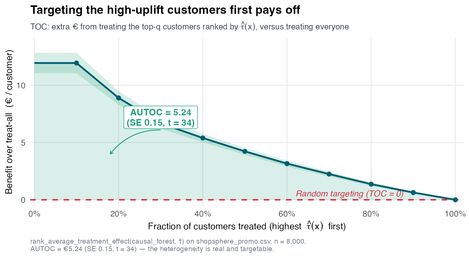
The split is deliberate — rank by \(\hat\tau\), score by \(\psi\): selecting the top-\(q\) with the prediction but evaluating it with an independent unbiased score (\(\mathbb{E}[\psi\mid X]=\tau(x)\)) avoids the circularity of letting the model grade its own homework — averaging \(\hat\tau\) itself within the top-\(q\) would flatter even an overfit ranking. Each \(\psi_i\) is very noisy, but the TOC reports group averages, so the noise washes out (hence the AUTOC’s \(t=34\) below), which is why the placebo — a random priority fed into the same machine, giving AUTOC ≈ 0 — is the decisive check that the curve is signal, not a wiggle a flexible learner draws from noise.
The RATE is the area under the TOC,
\[ \text{RATE} = \int_0^1 \mathrm{TOC}(q;\hat\tau)\,dq, \]
a positive value certifying that prioritizing by \(\hat\tau\) beats a blanket policy. Two cousins re-weight the same integral: the AUTOC is this uniform average (what grf reports by default, best when only a small fraction has large effects), while the QINI weights by \(q\), \(\int_0^1 q\,\mathrm{TOC}(q;\hat\tau)\,dq\), and works better when effects are more diffuse. On ShopSphere the TOC is steeply front-loaded (Figure 13.7): the AUTOC-style RATE = 5.24 (SE 0.15, \(t = 34\)), decisively positive (Python’s manual RATE 6.35 — an estimator-and-scale difference we document, not force-match). Together with the BLP we now hold both certificates: the heterogeneity is real and targeting it pays.
13.3.4.4 CLAN: who are the extremes, and the three-gate checklist
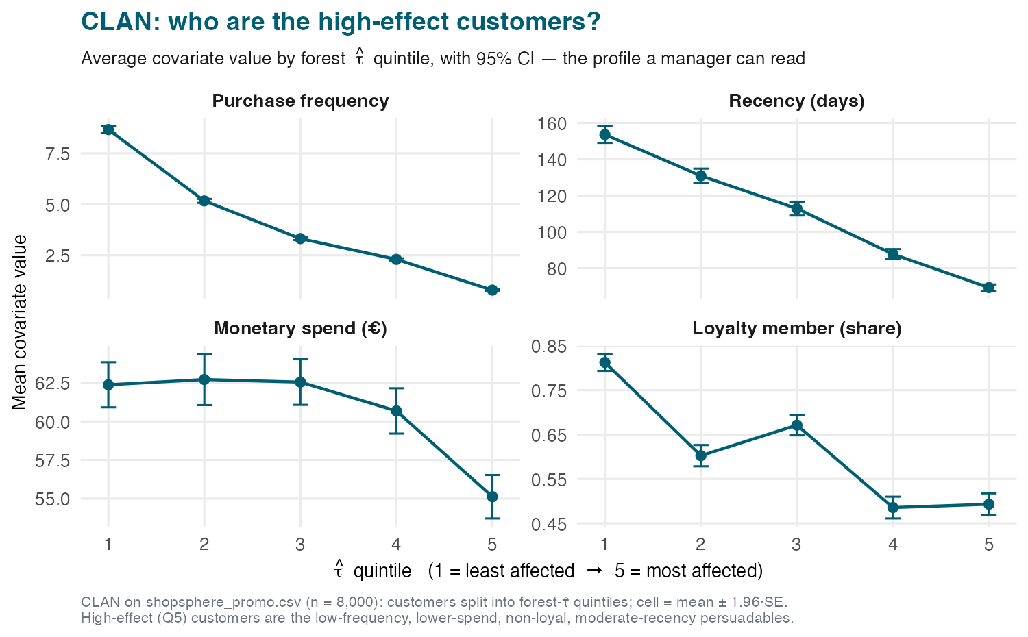
A validated \(\hat\tau(x)\) lets us characterize the high- and low-effect customers — Classification Analysis (CLAN) (Chernozhukov et al. 2018). Take the least-affected group \(G_1\) and most-affected group \(G_K\) from the sorted-group GATES and compare their average covariates, \(\delta_K - \delta_1\) with \(\delta_k = \mathbb{E}[X \mid G_k]\). On ShopSphere the high-effect group is the lapsing, low-frequency, low-engagement customers (the classic persuadables); the low-effect group is the loyal regulars who would buy anyway. This converts a black-box \(\hat\tau(x)\) into a describable persona (Figure 13.9) — and is a sanity check: if the extremes make no business sense, or contradict domain knowledge, distrust the model regardless of a significant BLP.
13.3.5 From estimate to decision: policy learning
13.3.5.1 The deliverable is a rule, and CATE accuracy is not policy quality
A manager cannot deploy a histogram. The deliverable is a policy \(\pi: X \to \{0,1\}\) that says, for each customer, treat or not. We judge it by its value — the expected outcome under deployment, \(V(\pi) = \mathbb{E}[Y(\pi(X))]\) — and seek the value-maximizing \(\pi\), possibly under constraints (budget, fairness, explainability). The naive rule treats customer \(i\) iff \(\hat\tau(X_i) > 0\). It is intuitive but flawed, because CATE accuracy and policy value reward different things (Qian and Murphy 2011). For the decision, all that matters is getting the sign right near the threshold \(\tau(x)=0\): an error far from zero costs MSE but never flips the decision, while a tiny error near zero is cheap for MSE but flips treat to don’t-treat — exactly where it hurts. So an estimator optimized for MSE wastes its accuracy budget far from the boundary and is sloppy where decisions are made. We should optimize the decision boundary directly, not threshold a noisy point estimate. (This mirrors the meta-learner lesson: minimizing arm-wise MSE is not the best way to minimize CATE-MSE, and minimizing CATE-MSE is not the best way to learn a policy.)
13.3.5.2 Policy = weighted classification on the score
The spine’s fourth appearance. Compare the policy value against a fair-coin-flip benchmark \(\pi^{\text{coin}}\sim\text{Bernoulli}(0.5)\) and the objective simplifies to a weighted classification problem:
\[ \begin{aligned} \pi^* &= \arg\max_\pi \mathbb{E}[Y(\pi)] = \arg\max_\pi \Big(\mathbb{E}[Y(\pi)] - \tfrac{1}{2}\mathbb{E}[Y(1)] - \tfrac{1}{2}\mathbb{E}[Y(0)]\Big) \\ &= \arg\max_\pi \mathbb{E}\big[\pi Y(1) + (1-\pi)Y(0)\big] - \tfrac{1}{2}\mathbb{E}[Y(1)] - \tfrac{1}{2}\mathbb{E}[Y(0)] \\ &= \arg\max_\pi \mathbb{E}\big[(\pi - \tfrac{1}{2})(Y(1) - Y(0))\big] \;=\; \arg\max_\pi \mathbb{E}\big[(2\pi - 1)(Y(1) - Y(0))\big] \\ &\overset{\text{LIE}}{=} \arg\max_\pi \mathbb{E}\big[(2\pi(X) - 1)\,\tau(X)\big] \;=\; \arg\max_\pi \underbrace{\mathbb{E}\big[|\tau(X)|\,\text{sign}(\tau(X))\,(2\pi(X) - 1)\big]}_{A(\pi),\ \text{the policy advantage}}. \end{aligned} \]
The advantage \(A(\pi)\) measures the gain over random allocation: if the policy picks the better treatment for \(X\) (\(\text{sign}(\tau(X))(2\pi(X)-1) = 1\)) we earn \(|\tau(X)|\); if it picks the worse one we lose \(|\tau(X)|\). So we must get it right for those with the biggest \(|\tau|\); units with CATEs near zero are negligible — the decision-loss logic of the previous paragraph, made formal, and the difference from CATE-MSE minimization, which demands good approximations everywhere. Since potential outcomes are unobserved, Athey and Wager (Athey and Wager 2021) recommend plugging in the AIPW score (again), turning the population objective into the empirical weighted classification problem
\[ \hat\pi = \arg\max_{\pi\in\Pi}\ \frac{1}{n}\sum_i \overbrace{|\psi_i|}^{\text{weight}}\,\underbrace{\text{sign}(\psi_i)}_{\text{label}}\,\overbrace{(2\pi(X_i) - 1)}^{\text{rule learned}} = \arg\max_{\pi\in\Pi}\ \frac{1}{n}\sum_i (2\pi(X_i) - 1)\,\psi_i. \]
When \(\psi_i > 0\) (the coupon helps \(i\)) the objective rewards treating; when \(\psi_i < 0\) it rewards withholding; units with large \(|\psi_i|\) dominate, so the policy concentrates correctness where the stakes are highest. Maximizing this doubly-robust value estimate targets policy value directly — no thresholding of a noisy \(\hat\tau\). Any classifier handling weighted classification works: decision trees/forests, logistic lasso, SVM.
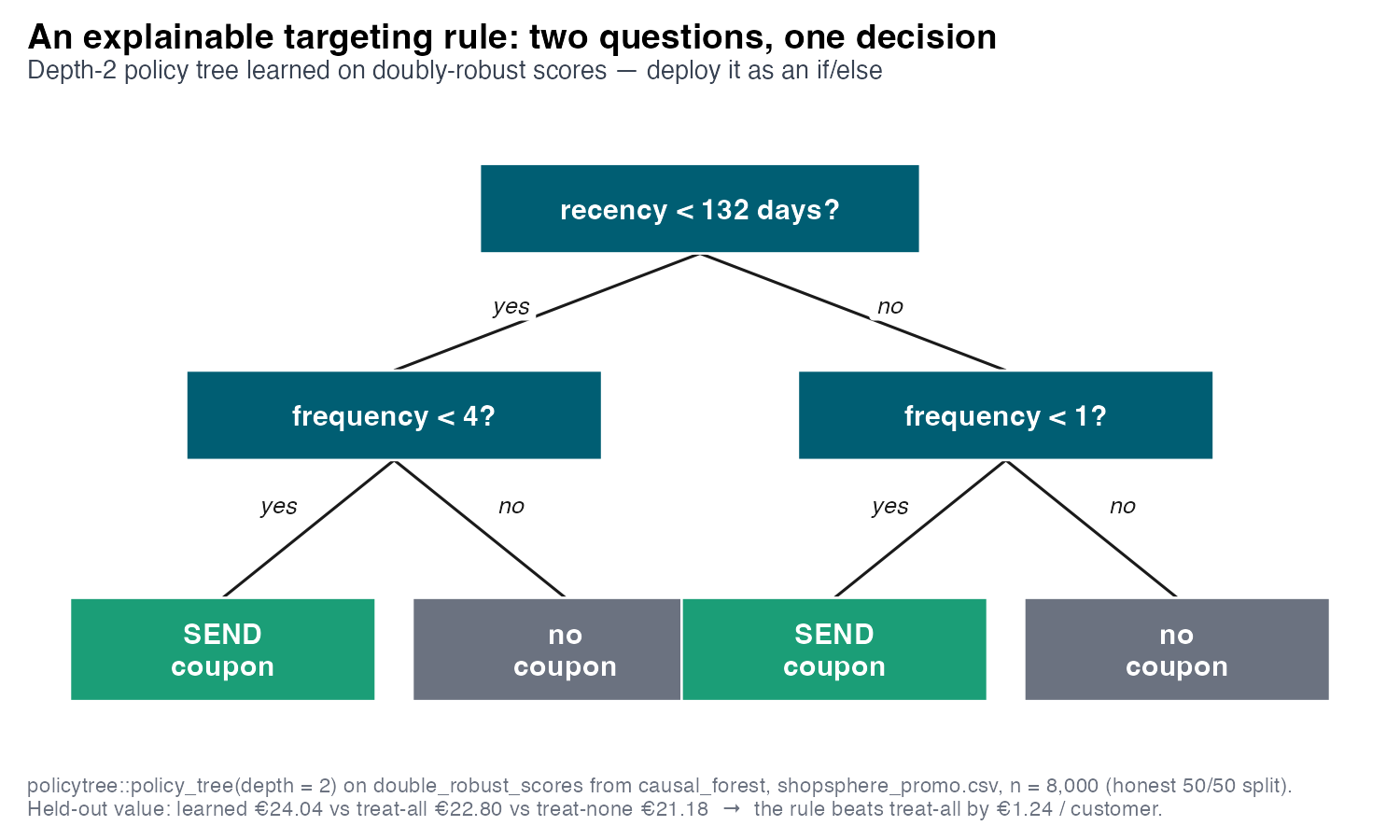
recency < 132 days; each branch then splits on frequency. Two leaves send the coupon — recency < 132 and frequency < 4 (the dominant cell), and recency ≥ 132 and frequency < 1 — the other two withhold. Held-out value: the rule yields €24.04 per customer versus €22.80 treat-all and €21.18 treat-none, beating the blanket campaign by +€1.24 / customer.
13.3.5.3 The policy tree: a rule you can defend
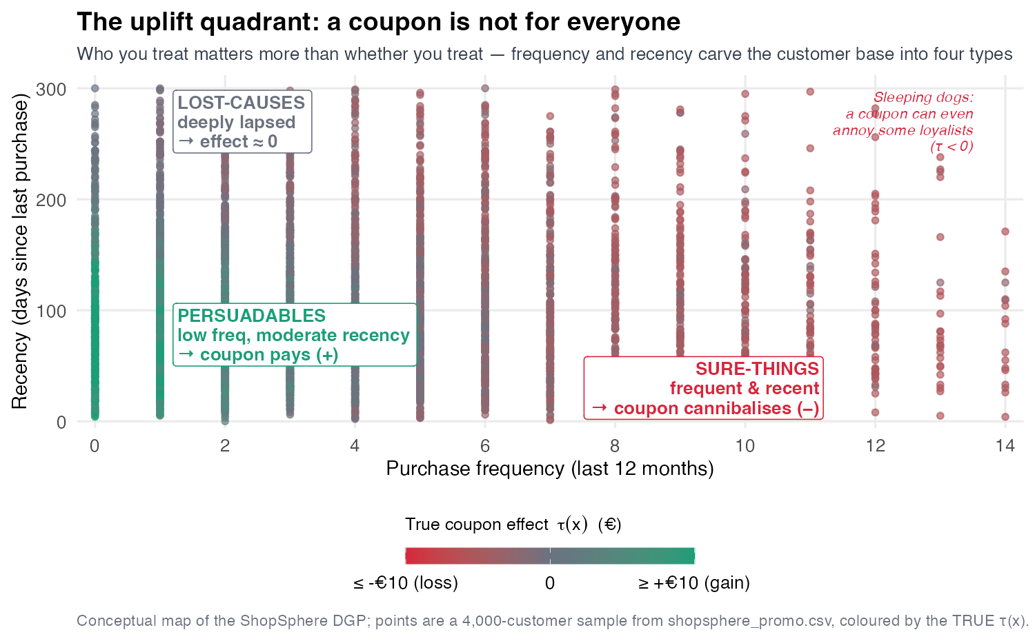
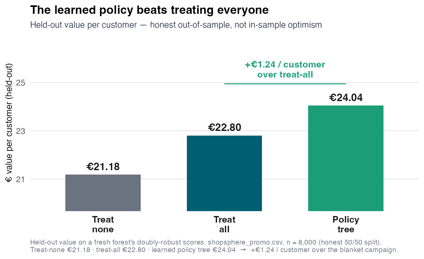
Restrict \(\pi\) to a shallow decision tree (Zhou, Athey, and Wager 2023) and the value-maximizing rule becomes human-readable. Constraining to depth 2 sacrifices a little value for enormous interpretability: the entire targeting rule is two questions. The learned tree on ShopSphere has two send-leaves (Figure 13.10): the dominant one is recency < 132 days and frequency < 4 purchases (recent but infrequent — reachable yet still persuadable), and a second small one is the lapsed near-one-timer (recency ≥ 132 and frequency < 1) — net-positive on average, because near-zero purchase frequency leaves no margin to cannibalize, so the coupon can only help (the truly deep-lapsed tail inside this leaf, recency ≳ 270, is the effect-≈0 “lost-cause” of Figure 13.2). Every other customer is withheld. The common thread is low frequency — leave the loyal regulars alone. It recovers the GATE story (effect falls with frequency) and the CLAN persona (persuadables are low-frequency) as an explicit, deployable rule. Evaluated on held-out data (so the value is honest, not in-sample optimism), the policy tree yields €24.04 per customer versus €22.80 treat-all and €21.18 treat-none — +€1.24 / customer over the blanket campaign (Figure 13.11). Python’s DRPolicyTree shows the same direction (+€0.20 on the effect scale; different estimator, same lesson).
13.3.6 Recap: one score, four jobs
Five load-bearing ideas carry the session. The average lies — a “meh” €1.4–1.5 ATE hid effects from −€6.5 to +€20.8, sign-flipping across customers. One score, four jobs — the S08 AIPW \(\psi_i\), with \(\mathbb{E}[\psi\mid X]=\tau(x)\): averaging it \(\to\) ATE was last week’s job; the four new jobs are group it \(\to\) GATE, regress on \(X\) \(\to\) \(\tau(x)\), rank it \(\to\) RATE, weight a classifier by it \(\to\) policy. Estimate with orthogonality — causal forests and the DR-learner target \(\tau\) directly; predicting \(Y\) well is not estimating \(\tau\) well. Validate before believing — a flexible learner always draws a wiggle, so clear BLP (real?), RATE (worth it?), CLAN (sensible?). Ship a rule, not a curve — policy is weighted classification on \(\psi\), and on ShopSphere the policy tree beat treat-all by +€1.24/customer.
S08 and S09 are one method seen twice: orthogonalize and cross-fit the score, then either average it (the ATE) or project it (heterogeneity, targeting, policy). Assignment IV spans both — de-confound an observational treatment, estimate and validate its heterogeneity, and recommend a targeting policy; the validation step is graded heavily because it is what separates a finding from a wiggle. The same orthogonal-score machinery returns in Part V, powering Chang’s double/debiased difference-in-differences (Chang 2020). The through-line of the whole course: identify the effect, estimate it honestly, then act on it.
13.4 Coding Lab
The lab works the ShopSphere coupon problem end to end on materials/data/shopsphere_promo.csv, a synthetic dataset where the truth is known — it is generated with a heterogeneous true \(\tau(x)\), true ATE = 1.69 — so each exercise is a recovery check, not a graded discovery (Assignment IV will use a different domain — FitLife — so nothing here pre-solves it). The arc follows the spine: build the GATE by hand from the S08 score, fit \(\tau(x)\) and check recovery, validate that the heterogeneity is real, then turn it into a policy. Each exercise gives a Scaffold with # ___ YOUR CODE placeholders in both R and Python; attempt it, then expand Show solution to compare. The solutions reproduce the locked numbers exactly; they are adapted from the verified pipelines in explorations/s09_verify.{R,py}.
Download the dataset: shopsphere_promo.csv
13.4.1 Exercise 1 — GATE by hand from the S08 score (~20 min)
The spine, second appearance. Cross-fit the AIPW score \(\psi_i\) exactly as in S08, then regress it on the frequency band to recover the GATEs with valid standard errors. The lesson: project \(\psi\) on a group \(G\) and the averages that hid the winners and losers split apart.
13.4.1.1 Scaffold
import numpy as np, pandas as pd
from sklearn.ensemble import RandomForestRegressor, RandomForestClassifier
from sklearn.model_selection import KFold
import statsmodels.api as sm

df = pd.read_csv("../../materials/data/shopsphere_promo.csv")
Xnum = ["recency","frequency","monetary","tenure","age","email_opens","loyalty_member"]
X = pd.get_dummies(df[Xnum + ["channel"]], columns=["channel"], drop_first=True).astype(float).values
Y = df["profit_30d"].values; T = df["coupon"].values.astype(int); n = len(Y)

# (a) 5-fold cross-fit mu1, mu0, e
mu1 = np.zeros(n); mu0 = np.zeros(n); e = np.zeros(n)
for tr, te in KFold(5, shuffle=True, random_state=7).split(X):
    # ___ YOUR CODE: fit RF on (X[tr][T[tr]==1], Y[tr][T[tr]==1]) -> mu1[te]; same for mu0
    # ___ YOUR CODE: fit RandomForestClassifier on (X[tr], T[tr]); e[te] = clip(predict_proba[:,1], .02, .98)
    pass

# (b) AIPW score and its mean (= ATE)
# ___ YOUR CODE: psi = mu1 - mu0 + T*(Y - mu1)/e - (1-T)*(Y - mu0)/(1-e); psi.mean()

# (c) regress psi on the frequency band -> GATE per band
band = pd.cut(df["frequency"], bins=[-1,1,3,6,np.inf], labels=["0-1","2-3","4-6","7+"])
# ___ YOUR CODE: Dband = pd.get_dummies(band).astype(float).values
# ___ YOUR CODE: sm.OLS(psi, Dband).fit(cov_type="HC3").summary()  # each coef is a GATE
TipShow solution
suppressPackageStartupMessages({
  library(readr); library(dplyr); library(ranger); library(estimatr)
})
set.seed(7)
df <- read_csv(here::here("materials/data/shopsphere_promo.csv"), show_col_types = FALSE)
Xdf <- df |> select(recency, frequency, monetary, tenure, age,
                    channel, email_opens, loyalty_member)
Y <- df$profit_30d; D <- df$coupon; n <- nrow(df); K <- 5

# --- 5-fold cross-fit the AIPW nuisances ---
fold <- sample(rep(1:K, length.out = n))
mu1 <- numeric(n); mu0 <- numeric(n); ehat <- numeric(n)
for (k in 1:K) {
  tr <- fold != k; te <- fold == k
  g1 <- ranger(x = Xdf[tr & D == 1, ], y = Y[tr & D == 1], num.trees = 800, min.node.size = 5)
  g0 <- ranger(x = Xdf[tr & D == 0, ], y = Y[tr & D == 0], num.trees = 800, min.node.size = 5)
  mm <- ranger(x = Xdf[tr, ],          y = D[tr],          num.trees = 800, min.node.size = 5)
  mu1[te]  <- predict(g1, Xdf[te, ])$predictions
  mu0[te]  <- predict(g0, Xdf[te, ])$predictions
  ehat[te] <- pmin(pmax(predict(mm, Xdf[te, ])$predictions, 0.02), 0.98)
}

# --- assemble the per-unit AIPW score; its mean is the ATE ---
psi <- (mu1 - mu0) + D * (Y - mu1) / ehat - (1 - D) * (Y - mu0) / (1 - ehat)
cat(sprintf("AIPW ATE (mean psi)   : %.3f  (SE %.3f)\n", mean(psi), sd(psi) / sqrt(n)))
AIPW ATE (mean psi) : 1.403 (SE 0.173)# --- regress psi on the frequency band: each coefficient is a GATE with a valid SE ---
band <- cut(df$frequency, breaks = c(-1, 1, 3, 6, Inf), labels = c("0-1", "2-3", "4-6", "7+"))
gate <- lm_robust(psi ~ 0 + band)
print(round(cbind(GATE = coef(gate),
SE = gate$std.error,
CI_lo = gate$conf.low, CI_hi = gate$conf.high), 2)) GATE SE CI_lo CI_hi
band0-1 8.13 0.35 7.44 8.81
band2-3 2.09 0.29 1.52 2.67
band4-6 -0.95 0.30 -1.53 -0.37
band7+ -4.54 0.41 -5.35 -3.73import numpy as np, pandas as pd
from sklearn.ensemble import RandomForestRegressor, RandomForestClassifier
from sklearn.model_selection import KFold
import statsmodels.api as sm
df = pd.read_csv("../../materials/data/shopsphere_promo.csv")
Xnum = ["recency","frequency","monetary","tenure","age","email_opens","loyalty_member"]
X = pd.get_dummies(df[Xnum + ["channel"]], columns=["channel"], drop_first=True).astype(float).values
Y = df["profit_30d"].values; T = df["coupon"].values.astype(int); n = len(Y)
# 5-fold cross-fit mu1, mu0, e
mu1 = np.zeros(n); mu0 = np.zeros(n); e = np.zeros(n)
for tr, te in KFold(5, shuffle=True, random_state=7).split(X):
g1 = RandomForestRegressor(n_estimators=800, min_samples_leaf=5, random_state=0).fit(X[tr][T[tr]==1], Y[tr][T[tr]==1])
g0 = RandomForestRegressor(n_estimators=800, min_samples_leaf=5, random_state=0).fit(X[tr][T[tr]==0], Y[tr][T[tr]==0])
mm = RandomForestClassifier(n_estimators=800, min_samples_leaf=5, random_state=0).fit(X[tr], T[tr])
mu1[te] = g1.predict(X[te]); mu0[te] = g0.predict(X[te])
e[te] = np.clip(mm.predict_proba(X[te])[:,1], 0.02, 0.98)
psi = mu1 - mu0 + T*(Y-mu1)/e - (1-T)*(Y-mu0)/(1-e)
print(f"AIPW ATE (mean psi) : {psi.mean():.3f} (SE {psi.std()/np.sqrt(n):.3f})")AIPW ATE (mean psi) : 1.519 (SE 0.166)# regress psi on the frequency band -> one GATE per band
band = pd.cut(df["frequency"], bins=[-1,1,3,6,np.inf], labels=["0-1","2-3","4-6","7+"])
Dband = pd.get_dummies(band)
ols = sm.OLS(psi, Dband.astype(float).values).fit(cov_type="HC3")
for name, b, se in zip(Dband.columns, ols.params, ols.bse):
print(f" GATE[{name:>3}] = {b:7.2f} (SE {se:.2f})") GATE[0-1] = 8.20 (SE 0.34)
GATE[2-3] = 2.09 (SE 0.29)
GATE[4-6] = -0.97 (SE 0.29)
GATE[ 7+] = -4.02 (SE 0.36)The score averages to the ATE (≈ €1.4–1.5), but projected on the frequency band it splits into roughly +€8 / +€2 / −€1 / −€4 (0–1, 2–3, 4–6, 7+) — tracking the locked true GATEs. Averaging collapsed a sign-changing distribution to its near-zero midpoint; the band-level projection recovers the winners and losers, each with an honest confidence interval. R and Python use independent random streams, so the last decimal differs — the monotone decline and the sign change do not.
13.4.2 Exercise 2 — Fit \(\tau(x)\): causal forest vs the meta-learner field (S/T/X/R/DR), and a recovery check (~40 min)
Estimate the continuous engine. A causal forest (grf) / CausalForestDML (econml) targets \(\tau\) directly; the plug-in meta-learners predict outcomes and subtract — the T-learner fits one model per arm, the S-learner fits a single model with the treatment folded in as a feature. Because the truth is known, plot estimate against the recomputed true \(\tau(x)\), read off the correlation, and compare the spread \(\text{sd}(\hat\tau)\) to the true 5.72. The forest should hug the line; the plug-ins should trail it and mis-scale the spread — watch the S-learner’s regularization shrink it. Then fit the DR-learner — Exercise 1’s AIPW score \(\psi\) regressed on the full covariate vector instead of on one group — the spine’s third job, and complete the field guide (Section 13.3.3.4) with two more: the X-learner (impute each unit’s effect from the other arm, then blend by the propensity) and the R-learner (the S08 Robinson residual-on-residual, now with a slope that varies in \(x\)). The lesson: target the causal quantity directly, but mind that no single learner dominates — tuning and implementation decide the finite-sample winner, and the causal forest tops both languages.
13.4.2.1 Scaffold
library(readr); library(dplyr); library(grf); library(ranger)
df <- read_csv(here::here("materials/data/shopsphere_promo.csv"), show_col_types = FALSE)
X <- model.matrix(~ 0 + recency + frequency + monetary + tenure + age +
                    email_opens + loyalty_member + channel, data = df)
Y <- df$profit_30d; W <- df$coupon

# recompute the TRUE tau(x) from the generator (recovery check only — not available in real life)
persuade <- 16 * exp(-df$frequency/3.0) * exp(-((df$recency-70)/85)^2) * (0.7 + 0.6*(df$monetary < 60))
cannibal <- 7.5 * (df$frequency/(df$frequency+4)) * (0.5 + 0.5*df$loyalty_member)
tau_true <- persuade - cannibal

# (a) causal forest -> tau_hat, then corr(tau_hat, tau_true)  (expect ~0.97)
set.seed(42)
# ___ YOUR CODE: cf <- causal_forest(X, Y, W, num.trees = 3000, honesty = TRUE)
# ___ YOUR CODE: tau_hat <- predict(cf)$predictions; cor(tau_hat, tau_true)

# (b) T-learner: a regression forest per arm, subtract (expect a LOWER corr, ~0.93)
# ___ YOUR CODE: rf1 <- regression_forest(X[W==1,], Y[W==1]); rf0 <- regression_forest(X[W==0,], Y[W==0])
# ___ YOUR CODE: tau_T <- predict(rf1, X)$predictions - predict(rf0, X)$predictions; cor(tau_T, tau_true)

# (c) S-learner: ONE forest with W as a feature, difference the two predictions
#     (corr ~0.94, but watch sd(tau_S) shrink BELOW the true 5.72 -> understated heterogeneity)
# ___ YOUR CODE: sf <- regression_forest(cbind(X, W = W), Y)
# ___ YOUR CODE: tau_S <- predict(sf, cbind(X, W = 1))$predictions - predict(sf, cbind(X, W = 0))$predictions
# ___ YOUR CODE: cor(tau_S, tau_true); sd(tau_S)

# (d) DR-learner: regress Exercise 1's AIPW score psi on the FULL X (Ex1 used ONE group -> GATE)
# ___ YOUR CODE: drf <- regression_forest(X, psi)            # psi carries over from Exercise 1
# ___ YOUR CODE: tau_DR <- predict(drf)$predictions; cor(tau_DR, tau_true)   # ~ the forest's 0.97

# (e) X-learner: impute each unit's effect via the OTHER arm, blend by propensity
#     (reuse the T-learner arms rf1/rf0 and Exercise 1's explicit propensity ehat)
# ___ YOUR CODE: imp1 <- Y[W==1] - predict(rf0, X[W==1,])$predictions   # treated:  Y - mu0(X)
# ___ YOUR CODE: imp0 <- predict(rf1, X[W==0,])$predictions - Y[W==0]   # control:  mu1(X) - Y
# ___ YOUR CODE: tau1 <- predict(regression_forest(X[W==1,], imp1), X)$predictions  # and tau0 likewise
# ___ YOUR CODE: tau_X <- ehat * tau0 + (1 - ehat) * tau1; cor(tau_X, tau_true)

# (f) R-learner: Robinson residuals -> weighted regression of the pseudo-outcome (slope varies in x)
#     l_hat = E[Y|X] FROM SCRATCH (like S08's PLR: regress Y on X, 5-fold cross-fit on Ex1's `fold`); reuse Ex1's ehat
# ___ YOUR CODE: l_hat <- numeric(n); for (k in 1:K) { tr <- fold!=k; te <- fold==k
# ___ YOUR CODE:   l_hat[te] <- predict(ranger(x=Xdf[tr,], y=Y[tr], num.trees=800, min.node.size=5), Xdf[te,])$predictions }
# ___ YOUR CODE: Ytil <- Y - l_hat; Dtil <- W - ehat
# ___ YOUR CODE: rlf <- regression_forest(X, Ytil/Dtil, sample.weights = Dtil^2); tau_R <- predict(rlf, X)$predictions; cor(tau_R, tau_true)
import numpy as np, pandas as pd
from sklearn.ensemble import RandomForestRegressor, RandomForestClassifier
df = pd.read_csv("../../materials/data/shopsphere_promo.csv")
Xnum = ["recency","frequency","monetary","tenure","age","email_opens","loyalty_member"]
X = pd.get_dummies(df[Xnum + ["channel"]], columns=["channel"], drop_first=True).astype(float).values
Y = df["profit_30d"].values; T = df["coupon"].values.astype(int)
persuade = 16*np.exp(-df.frequency/3.0)*np.exp(-((df.recency-70)/85)**2)*(0.7+0.6*(df.monetary<60))
cannibal = 7.5*(df.frequency/(df.frequency+4))*(0.5+0.5*df.loyalty_member)
tau_true = (persuade - cannibal).values
# (a) CausalForestDML -> effect(X); corr with tau_true (expect ~0.97)
from econml.dml import CausalForestDML
# ___ YOUR CODE: cf = CausalForestDML(model_y=RandomForestRegressor(...), model_t=RandomForestClassifier(...), discrete_treatment=True,
# n_estimators=3000, random_state=42); cf.fit(Y, T, X=X)
# ___ YOUR CODE: tau_hat = cf.effect(X); np.corrcoef(tau_hat, tau_true)[0,1]
# (b) T-learner -> effect(X); corr with tau_true (LOWER, RF-default gap vs grf)
from econml.metalearners import TLearner
# ___ YOUR CODE: tl = TLearner(models=RandomForestRegressor(...)); tl.fit(Y, T, X=X); tau_T = tl.effect(X)
# (c) S-learner -> effect(X); one model with T folded in (corr below CF; tighter spread than T)
from econml.metalearners import SLearner
# ___ YOUR CODE: sl = SLearner(overall_model=RandomForestRegressor(...)); sl.fit(Y, T, X=X); tau_S = sl.effect(X)
# ___ YOUR CODE: np.corrcoef(tau_S, tau_true)[0,1]; tau_S.std()
# (d) DR-learner -> effect(X): regress the AIPW score on X (econml builds the cross-fit score internally)
from econml.dr import DRLearner
# ___ YOUR CODE: drl = DRLearner(model_regression=RandomForestRegressor(...), model_propensity=RandomForestClassifier(...)); drl.fit(Y, T, X=X)
# ___ YOUR CODE: tau_DR = drl.effect(X); np.corrcoef(tau_DR, tau_true)[0,1] # orthogonal; econml defaults trail CF here
# (e) X-learner -> effect(X): impute via the other arm, blend by propensity
from econml.metalearners import XLearner
# ___ YOUR CODE: xl = XLearner(models=RandomForestRegressor(...), propensity_model=RandomForestClassifier(...)); xl.fit(Y, T, X=X)
# ___ YOUR CODE: tau_X = xl.effect(X); np.corrcoef(tau_X, tau_true)[0,1] # strong even at 50/50 balance
# (f) R-learner -> effect(X): Robinson residual-on-residual with a varying slope
from econml.dml import NonParamDML
# ___ YOUR CODE: rl = NonParamDML(model_y=RandomForestRegressor(...), model_t=RandomForestClassifier(...), model_final=RandomForestRegressor(...), discrete_treatment=True); rl.fit(Y, T, X=X)
# ___ YOUR CODE: tau_R = rl.effect(X); np.corrcoef(tau_R, tau_true)[0,1] # econml default final trails (like DR)
TipShow solution
suppressPackageStartupMessages({ library(readr); library(dplyr); library(grf); library(ranger) })
df <- read_csv(here::here("materials/data/shopsphere_promo.csv"), show_col_types = FALSE)
X <- model.matrix(~ 0 + recency + frequency + monetary + tenure + age +
                    email_opens + loyalty_member + channel, data = df)
Y <- df$profit_30d; W <- df$coupon

persuade <- 16 * exp(-df$frequency/3.0) * exp(-((df$recency-70)/85)^2) * (0.7 + 0.6*(df$monetary < 60))
cannibal <- 7.5 * (df$frequency/(df$frequency+4)) * (0.5 + 0.5*df$loyalty_member)
tau_true <- persuade - cannibal

# --- causal forest: targets tau directly ---
set.seed(42)
cf <- causal_forest(X, Y, W, num.trees = 3000, honesty = TRUE)
tau_hat <- predict(cf)$predictions
ate <- average_treatment_effect(cf, target.sample = "all")
cat(sprintf("[CF] ATE (AIPW)             : %.3f  (SE %.3f)\n", ate[1], ate[2]))
[CF] ATE (AIPW) : 1.385 (SE 0.160)cat(sprintf("[CF] corr(tau_hat, tau_true): %.3f\n", cor(tau_hat, tau_true)))[CF] corr(tau_hat, tau_true): 0.970cat(sprintf("[CF] tau_hat range : [%.2f, %.2f] (true [%.2f, %.2f])\n",
min(tau_hat), max(tau_hat), min(tau_true), max(tau_true)))[CF] tau_hat range : [-4.98, 16.97] (true [-6.53, 20.80])# --- T-learner: regression forest per arm, subtract (noisier) ---
rf1 <- regression_forest(X[W == 1, ], Y[W == 1])
rf0 <- regression_forest(X[W == 0, ], Y[W == 0])
tau_T <- predict(rf1, X)$predictions - predict(rf0, X)$predictions
cat(sprintf("[T ] corr(tau_T, tau_true): %.3f sd %.2f (T-learner, lower corr)\n",
cor(tau_T, tau_true), sd(tau_T)))[T ] corr(tau_T, tau_true): 0.932 sd 5.77 (T-learner, lower corr)# --- S-learner: one forest with W as a feature; regularization compresses the effect ---
sf <- regression_forest(cbind(X, W = W), Y)
tau_S <- predict(sf, cbind(X, W = 1))$predictions - predict(sf, cbind(X, W = 0))$predictions
cat(sprintf("[S ] corr(tau_S, tau_true): %.3f sd %.2f (vs true sd %.2f -> understated)\n",
cor(tau_S, tau_true), sd(tau_S), sd(tau_true)))[S ] corr(tau_S, tau_true): 0.937 sd 4.33 (vs true sd 5.72 -> understated)# --- DR-learner: regress Exercise 1's AIPW score psi on the full X (the spine's 3rd job) ---
drf <- regression_forest(X, psi) # psi carries over from Exercise 1
tau_DR <- predict(drf)$predictions
cat(sprintf("[DR] corr(tau_DR, tau_true): %.3f sd %.2f (matches CF -> same orthogonal target)\n",
cor(tau_DR, tau_true), sd(tau_DR)))[DR] corr(tau_DR, tau_true): 0.967 sd 5.23 (matches CF -> same orthogonal target)# --- X-learner: impute each unit's effect via the OTHER arm, then blend by the propensity ---
# reuses the T-learner arms (rf1, rf0) and Exercise 1's explicit propensity (ehat = E[D|X])
mu1_all <- predict(rf1, X)$predictions # treated-arm outcome model
mu0_all <- predict(rf0, X)$predictions # control-arm outcome model
imp1 <- Y[W == 1] - mu0_all[W == 1] # treated: Y - mu0(X)
imp0 <- mu1_all[W == 0] - Y[W == 0] # control: mu1(X) - Y
tau1 <- predict(regression_forest(X[W == 1, ], imp1), X)$predictions # treated-arm CATE
tau0 <- predict(regression_forest(X[W == 0, ], imp0), X)$predictions # control-arm CATE
tau_X <- ehat * tau0 + (1 - ehat) * tau1 # blend by Ex1's propensity (leans on larger arm)
cat(sprintf("[X ] corr(tau_X, tau_true): %.3f sd %.2f (imputed + blended; here ~ the forest)\n",
cor(tau_X, tau_true), sd(tau_X)))[X ] corr(tau_X, tau_true): 0.967 sd 5.10 (imputed + blended; here ~ the forest)# --- R-learner: Robinson residuals -> weighted regression of the pseudo-outcome (varying slope) ---
# l_hat = E[Y|X] built FROM SCRATCH -- exactly S08's PLR nuisance: regress Y on X over ALL units,
# 5-fold cross-fit reusing Exercise 1's fold split; ehat = E[D|X] reused from Ex1 (one propensity lab-wide).
l_hat <- numeric(n) # reduced-form outcome predictor E[Y|X] (S08's ml_l)
for (k in 1:K) { # same 5 folds as the AIPW nuisances
tr <- fold != k; te <- fold == k
fY <- ranger(x = Xdf[tr, ], y = Y[tr], num.trees = 800, min.node.size = 5)
l_hat[te] <- predict(fY, Xdf[te, ])$predictions
}
Ytil <- Y - l_hat # outcome residual (Robinson; S08's res_y)
Dtil <- W - ehat # treatment residual (Ex1's propensity)
rlf <- regression_forest(X, Ytil / Dtil, sample.weights = Dtil^2) # weight = (D - e)^2; slope varies in x
tau_R <- predict(rlf, X)$predictions
cat(sprintf("[R ] corr(tau_R, tau_true): %.3f sd %.2f (orthogonal residuals -> targets tau)\n",
cor(tau_R, tau_true), sd(tau_R)))[R ] corr(tau_R, tau_true): 0.955 sd 5.24 (orthogonal residuals -> targets tau)plot(tau_true, tau_hat, pch = 19, col = "#00C1D466", cex = 0.4,
xlab = "true tau(x)", ylab = "estimated tau-hat(x)",
main = "Causal forest recovers the true effect")
abline(0, 1, lty = 2, col = "grey40")
import numpy as np, pandas as pd
from sklearn.ensemble import RandomForestRegressor, RandomForestClassifier
df = pd.read_csv("../../materials/data/shopsphere_promo.csv")
Xnum = ["recency","frequency","monetary","tenure","age","email_opens","loyalty_member"]
X = pd.get_dummies(df[Xnum + ["channel"]], columns=["channel"], drop_first=True).astype(float).values
Y = df["profit_30d"].values; T = df["coupon"].values.astype(int)

persuade = 16*np.exp(-df.frequency/3.0)*np.exp(-((df.recency-70)/85)**2)*(0.7+0.6*(df.monetary<60))
cannibal = 7.5*(df.frequency/(df.frequency+4))*(0.5+0.5*df.loyalty_member)
tau_true = (persuade - cannibal).values

from econml.dml import CausalForestDML
cf = CausalForestDML(model_y=RandomForestRegressor(n_estimators=400, min_samples_leaf=5, random_state=0),
                     model_t=RandomForestClassifier(n_estimators=400, min_samples_leaf=5, random_state=0),
                     discrete_treatment=True, n_estimators=3000, random_state=42)
cf.fit(Y, T, X=X)
<econml.dml.causal_forest.CausalForestDML object at 0x11f869d30>tau_hat = cf.effect(X)
print(f"[CF] ATE : {cf.ate(X):.3f}")[CF] ATE : 1.507print(f"[CF] corr(tau_hat,tau_true) : {np.corrcoef(tau_hat, tau_true)[0,1]:.3f}")[CF] corr(tau_hat,tau_true) : 0.967print(f"[CF] tau_hat range : [{tau_hat.min():.2f}, {tau_hat.max():.2f}]")[CF] tau_hat range : [-6.47, 17.84]from econml.metalearners import TLearner, SLearner
tl = TLearner(models=RandomForestRegressor(n_estimators=400, min_samples_leaf=5, random_state=0))
tl.fit(Y, T, X=X)<econml.metalearners._metalearners.TLearner object at 0x11f86b4d0>tau_T = tl.effect(X)
print(f"[T ] corr(tau_T, tau_true) : {np.corrcoef(tau_T, tau_true)[0,1]:.3f} sd {tau_T.std():.2f} (lower than CF)")[T ] corr(tau_T, tau_true) : 0.879 sd 6.36 (lower than CF)# S-learner: one model with T folded in -> tightest spread of the three
sl = SLearner(overall_model=RandomForestRegressor(n_estimators=400, min_samples_leaf=5, random_state=0))
sl.fit(Y, T, X=X)<econml.metalearners._metalearners.SLearner object at 0x11f86ae40>tau_S = sl.effect(X)
print(f"[S ] corr(tau_S, tau_true) : {np.corrcoef(tau_S, tau_true)[0,1]:.3f} sd {tau_S.std():.2f} (vs true sd {tau_true.std():.2f})")[S ] corr(tau_S, tau_true) : 0.901 sd 5.29 (vs true sd 5.72)# DR-learner: regress the AIPW score on X (econml cross-fits the score internally) -> matches CF
from econml.dr import DRLearner
drl = DRLearner(model_regression=RandomForestRegressor(n_estimators=400, min_samples_leaf=5, random_state=0),
model_propensity=RandomForestClassifier(n_estimators=400, min_samples_leaf=5, random_state=0),
random_state=0)
drl.fit(Y, T, X=X)<econml.dr._drlearner.DRLearner object at 0x11f86b620>tau_DR = drl.effect(X)
print(f"[DR] corr(tau_DR, tau_true) : {np.corrcoef(tau_DR, tau_true)[0,1]:.3f} sd {tau_DR.std():.2f} (orthogonal, but econml defaults trail CF here)")[DR] corr(tau_DR, tau_true) : 0.808 sd 4.68 (orthogonal, but econml defaults trail CF here)# X-learner: impute via the other arm, blend by the propensity -> strong even at 50/50 balance
from econml.metalearners import XLearner
xl = XLearner(models=RandomForestRegressor(n_estimators=400, min_samples_leaf=5, random_state=0),
propensity_model=RandomForestClassifier(n_estimators=400, min_samples_leaf=5, random_state=0))
xl.fit(Y, T, X=X)<econml.metalearners._metalearners.XLearner object at 0x11f86bcb0>tau_X = xl.effect(X)
print(f"[X ] corr(tau_X, tau_true) : {np.corrcoef(tau_X, tau_true)[0,1]:.3f} sd {tau_X.std():.2f} (imputed + blended)")[X ] corr(tau_X, tau_true) : 0.950 sd 5.69 (imputed + blended)# R-learner: Robinson residual-on-residual with a varying slope (NonParamDML = the R-learner)
from econml.dml import NonParamDML
rl = NonParamDML(model_y=RandomForestRegressor(n_estimators=400, min_samples_leaf=5, random_state=0),
model_t=RandomForestClassifier(n_estimators=400, min_samples_leaf=5, random_state=0),
model_final=RandomForestRegressor(n_estimators=400, min_samples_leaf=5, random_state=0),
discrete_treatment=True, random_state=0)
rl.fit(Y, T, X=X)<econml.dml.dml.NonParamDML object at 0x11f86acf0>tau_R = rl.effect(X)
print(f"[R ] corr(tau_R, tau_true) : {np.corrcoef(tau_R, tau_true)[0,1]:.3f} sd {tau_R.std():.2f} (econml default final trails, like DR)")[R ] corr(tau_R, tau_true) : 0.754 sd 7.57 (econml default final trails, like DR)The causal forest tracks the truth at corr ≈ 0.97 (R 0.970, Python 0.967) and its AIPW ATE recovers the de-confounded average (≈ €1.4–1.5 — the same ballpark as Exercise 1’s AIPW estimate, and nowhere near the sign-flipped naive −1.38). Both plug-in meta-learners trail it: the T-learner lands at ≈ 0.93 in R (0.932) and ≈ 0.88 in Python (0.879), and the S-learner at ≈ 0.94 in R (0.937) and ≈ 0.90 in Python (0.901) — econml’s default per-arm forests are tuned differently from grf, the documented parity gap, not a bug. Correlation is only half the story, though — look at the spread. The S-learner produces the tightest \(\hat\tau\) of the three: it folds \(D\) into one regularized model that shrinks the weak treatment signal, so in grf its standard deviation collapses to 4.33, well below the true 5.72 — the textbook “regularization understates heterogeneity.” The T-learner does not compress: its spread (sd 5.77) sits right at the true 5.72 — but its two independently-tuned forests buy that magnitude with estimation noise (a heavier lower tail), not calibrated signal, which is why its ranking still trails the forest at corr 0.93. Only the forest, which targets the difference directly (its local moment), recovers both a faithful ranking and a calibrated spread (sd ≈ 5.0) — exactly as the MCE decomposition predicts. The DR-learner closes the field guide: regress Exercise 1’s same score \(\psi\) on the full covariate vector (rather than on one frequency band). In R it lands at corr 0.967, essentially the causal forest’s 0.970 — the grf forest is a DR-learner with a learned neighbourhood weighting, so the notes’ claim that the two “fit the same orthogonal target” (Section 13.3.3.4) is shown, not asserted. econml’s generic DRLearner is the instructive counterpoint: with its default model_final it trails at 0.808, below even the plug-in S/T here — a concrete reminder that no single learner dominates (Section 13.3.3.4). Orthogonality is the right principle; the forest’s honest-splitting, local-moment machinery is what makes it the robust winner on this surface. We document the gap rather than force-match it.
Two more learners close the field guide. The X-learner builds straight on the T-learner — imputing each unit’s effect from the opposite arm, then blending the two by the propensity — and recovers at corr 0.967 in R and 0.950 in Python: essentially the forest (and matching the DR-learner), and well above the raw T-learner it extends. The cross-arm imputation denoises exactly the two-independent-forests gap that held the T-learner back — even though ShopSphere’s 50/50 balance never triggers the X-learner’s headline imbalance advantage, so its real virtue stays a named use-case here, not a demonstrated win. The R-learner — Robinson’s residual-on-residual with a slope that varies in \(x\) — is last week’s partially-linear model put to local use: we cross-fit \(\hat\ell=\mathbb{E}[Y\mid X]\) from scratch (regress \(Y\) on \(X\) over all units, the same 5-fold split as Exercise 1 — exactly S08’s ml_l nuisance) and reuse Exercise 1’s propensity \(\hat e\), then fit a \(\tilde D^2\)-weighted forest of the pseudo-outcome \(\tilde Y/\tilde D\) on \(X\). It lands at corr 0.955 in R, just below the forest. Under econml’s NonParamDML with a default random-forest final stage it trails at 0.754 (spread inflated to sd ≈ 7.6), the same defaults-trail story as the DR-learner: the weighted pseudo-outcome regression is high-variance unless its final learner is tuned. That is the whole lesson in one panel — an orthogonal score targeting \(\tau\) is the right principle (in R the forest, DR-, R-, and even the imputed-and-blended X-learner all cluster at 0.96–0.97), but the finite-sample winner is decided by the final-stage learner and its tuning: econml’s generic finals leave both the R- and DR-learners behind, while grf’s honest, locally-weighted machinery does not. Read the gap; don’t force-match it.
13.4.3 Exercise 3 — Validate the estimate: BLP, RATE/TOC, and CLAN (~35 min)
Validate before believing — the three gates. Run grf’s test_calibration (the BLP/calibration test) and best_linear_projection, then rank_average_treatment_effect for the RATE/AUTOC, and finally CLAN — compare the covariate means of the most- and least-affected \(\hat\tau\) deciles; in Python, build the AIPW score, regress it on the demeaned \(\hat\tau\) for the BLP \(\beta_2\), integrate a manual TOC, and run the same decile comparison. The lesson: the wide histogram is signal, not noise (real?); the ranking pays (worth it?); and the extremes resolve into personas a manager recognizes (sensible?). Each step also gets a picture: a who-benefits scatter (\(\hat\tau\) vs frequency), the TOC curve (grf’s plot(rate) draws it for free), and the CLAN profile — average covariate by \(\hat\tau\) quintile with 95% CI, the real result that replaces a hand-drawn persona map. We run every gate twice, side by side — for the forest’s tau_hat and the DR-learner’s tau_DR from Exercise 2 — to make the deeper point concrete: validation lives on the orthogonal score \(\psi\), not on grf. rank_average_treatment_effect accepts any estimator’s ranking through its priorities argument, and the calibration \(\beta_2\) is a one-line lm_robust of \(\psi\) on the demeaned estimate. The DR-learner clears all three gates in both languages — in R within a hair of the forest, but in Python with a visibly lower AUTOC because econml’s default DR-learner ranks less sharply (the documented ~0.81 trail). That is validation doing its job: it certifies the heterogeneity is real and measures that one estimator’s targeting is worth less than another’s.
13.4.3.1 Scaffold
# Reuses cf, tau_hat, tau_DR (Ex2) and psi (Ex1). Validate BOTH estimators side by side:
#   tau_hat via grf's functions; tau_DR via the SAME checks on the score psi.

# (a) calibration beta2 (is the ranking real?): ~1, p tiny -- for EACH estimator
# ___ YOUR CODE: test_calibration(cf)                                # tau_hat: grf reads its own scores
# ___ YOUR CODE: lm_robust(psi ~ I(tau_DR - mean(tau_DR)))          # tau_DR: the slope IS beta2

# (b) best linear projection on the two dominant modifiers (estimator-agnostic -- it projects the score)
# ___ YOUR CODE: best_linear_projection(cf, X[, c("frequency","recency")])  # or: lm_robust(psi ~ frequency + recency)

# (c) RATE / AUTOC (is it worth it?, expect ~5.2). rank_average_treatment_effect takes ANY ranking as `priorities`:
# ___ YOUR CODE: rank_average_treatment_effect(cf, tau_hat)$estimate   # rank by the forest
# ___ YOUR CODE: rank_average_treatment_effect(cf, tau_DR)$estimate    # rank by the DR-learner (cf supplies the scores)

# (d) CLAN (is it sensible?): mean covariates of the most- vs least-affected decile -- for EACH estimator
# ___ YOUR CODE: hi <- tau_hat >= quantile(tau_hat, .9); lo <- tau_hat <= quantile(tau_hat, .1)   # repeat with tau_DR
# ___ YOUR CODE: compare column means of df[hi, c("frequency","recency","monetary","loyalty_member")] vs df[lo, ]

# (e) PLOTS: who-benefits scatter + the TOC curve + the CLAN profile (on tau_hat)
# ___ YOUR CODE: plot(df$frequency, tau_hat); lines(lowess(df$frequency, tau_hat))   # who benefits
# ___ YOUR CODE: plot(rank_average_treatment_effect(cf, tau_hat))                    # grf draws the TOC for you
# ___ YOUR CODE: ntile(tau_hat, 5) -> mean of each covariate per quintile (+95% CI) -> facet_wrap   # CLAN profile
# Reuses X, Y, T, tau_hat from Exercise 2 (econml has no test_calibration -> do it manually)
import statsmodels.api as sm
from sklearn.model_selection import KFold
# Validate BOTH tau_hat and tau_DR (Ex2) side by side -- the same manual checks on the score psi.
# (a) build a cross-fitted AIPW score psi, then the calibration beta2 = slope of psi on the demeaned estimate
# ___ YOUR CODE: cross-fit mu1, mu0, e (as in Ex1); psi = mu1-mu0 + T*(Y-mu1)/e - (1-T)*(Y-mu0)/(1-e)
# ___ YOUR CODE: for tau in (tau_hat, tau_DR): sm.OLS(psi, sm.add_constant(tau - tau.mean())).fit(cov_type="HC3").params[1]
# (b) BLP gradient on psi (what drives it? -- estimator-agnostic): regress psi on frequency + recency
# ___ YOUR CODE: sm.OLS(psi, sm.add_constant(df[["frequency","recency"]].values)).fit(cov_type="HC3").params[1:]
# (c) manual AUTOC (is it worth it?): sort psi by the estimate, cumulative-mean minus ATE, average -- for EACH
# ___ YOUR CODE: order = np.argsort(-tau); np.mean([psi[order][:k].mean() - psi.mean() for k in 1..n]) # tau_hat & tau_DR
# (d) CLAN ("is it sensible?"): mean covariates of the most- vs least-affected decile -- for EACH estimator
# ___ YOUR CODE: hi = tau >= np.quantile(tau, .9); lo = tau <= np.quantile(tau, .1) # repeat for tau_hat and tau_DR
# ___ YOUR CODE: for cols frequency/recency/monetary/loyalty_member, compare df[c][hi].mean() vs df[c][lo].mean()
# (d) PLOTS (matplotlib): who-benefits scatter + the manual TOC curve + the CLAN profile
# ___ YOUR CODE: plt.scatter(df.frequency, tau_hat) + a binned-mean trend # who benefits
# ___ YOUR CODE: plt.plot(q_grid, toc) and the random placebo toc_r # TOC curve
# ___ YOUR CODE: pd.qcut(tau_hat,5) -> mean of each covariate per quintile (+95% CI) -> 2x2 subplots # CLAN profile
TipShow solution
suppressPackageStartupMessages({ library(grf); library(estimatr) })
# Reuses cf, tau_hat, tau_DR (Ex2) and psi (Ex1). We validate BOTH estimators side by side:
#   tau_hat = causal forest -> grf's built-ins read its own scores
#   tau_DR  = DR-learner     -> the SAME checks, by hand on the orthogonal score psi
# The point: validation lives on the score psi, not on grf -- any IATE validates the same way.

# (a) Is the heterogeneity real? -- the calibration coefficient beta2 (~1, p tiny)
cat("[CAL] tau_cf  test_calibration(cf):\n")
[CAL] tau_cf test_calibration(cf):print(round(test_calibration(cf), 4)) # differential.forest.prediction = beta2
Best linear fit using forest predictions (on held-out data)
as well as the mean forest prediction as regressors, along
with one-sided heteroskedasticity-robust (HC3) SEs:

                               Estimate Std. Error t value    Pr(>t)
mean.forest.prediction           0.9554     0.1034  9.2375 < 2.2e-16 ***
differential.forest.prediction   1.0800     0.0295 36.5661 < 2.2e-16 ***
---
Signif. codes:  0 '***' 0.001 '**' 0.01 '*' 0.05 '.' 0.1 ' ' 1
cal_dr <- lm_robust(psi ~ I(tau_DR - mean(tau_DR))) # SAME test by hand: regress psi on demeaned tau_DR
cat(sprintf("[CAL] tau_DR by-hand: beta1 = %.3f (= AIPW ATE) beta2 = %.3f (SE %.3f, t = %.1f)\n",
coef(cal_dr)[1], coef(cal_dr)[2], cal_dr$std.error[2], coef(cal_dr)[2] / cal_dr$std.error[2]))[CAL] tau_DR by-hand: beta1 = 1.403 (= AIPW ATE) beta2 = 1.042 (SE 0.033, t = 31.4)# (b) What drives it? -- best linear projection on the dominant modifiers (estimator-agnostic: projects the score)
cat("\n[BLP] tau_cf best_linear_projection(cf, frequency + recency):\n")
[BLP] tau_cf best_linear_projection(cf, frequency + recency):print(best_linear_projection(cf, X[, c("frequency", "recency")]))
Best linear projection of the conditional average treatment effect.
Confidence intervals are cluster- and heteroskedasticity-robust (HC3):

              Estimate Std. Error t value  Pr(>|t|)
(Intercept)  9.2770812  0.3426184  27.077 < 2.2e-16 ***
frequency   -1.1880879  0.0510726 -23.263 < 2.2e-16 ***
recency     -0.0277993  0.0019723 -14.095 < 2.2e-16 ***
---
Signif. codes:  0 '***' 0.001 '**' 0.01 '*' 0.05 '.' 0.1 ' ' 1
bd <- data.frame(psi = psi, frequency = df$frequency, recency = df$recency)
blp_hand <- lm_robust(psi ~ frequency + recency, data = bd) # the same projection on our own score psi
cat(sprintf("[BLP] by-hand on psi: frequency = %.3f (SE %.3f), recency = %.4f (SE %.4f) -- same gradient\n",
coef(blp_hand)[2], blp_hand$std.error[2], coef(blp_hand)[3], blp_hand$std.error[3]))[BLP] by-hand on psi: frequency = -1.269 (SE 0.069), recency = -0.0276 (SE 0.0021) -- same gradient# Modifier scatter: tau_hat vs the dominant modifier — the BLP gradient, drawn ("who benefits")
plot(df$frequency, tau_hat, pch = 19, col = "#00C1D433", cex = 0.4,
xlab = "purchase frequency", ylab = expression(hat(tau)(x)),
main = "Who benefits: effect falls with frequency")
abline(h = 0, lty = 3, col = "grey50")
lines(lowess(df$frequency, tau_hat), col = "#005e73", lwd = 2.5)
# (c) Is it worth it? -- RATE / AUTOC. rank_average_treatment_effect takes ANY ranking as `priorities`,
#     so pass tau_DR to validate the DR-learner's targeting (cf only supplies the evaluation scores).
rate_cf <- rank_average_treatment_effect(cf, tau_hat)
rate_dr <- rank_average_treatment_effect(cf, tau_DR)
set.seed(99)
rate_rand <- rank_average_treatment_effect(cf, runif(nrow(X)))   # placebo: a meaningless (random) priority
cat(sprintf("\n[RATE] AUTOC  tau_cf = %.3f (t = %.1f)   tau_DR = %.3f (t = %.1f)   placebo = %.3f (SE %.3f -> CI covers 0)\n",
            rate_cf$estimate, rate_cf$estimate / rate_cf$std.err,
            rate_dr$estimate, rate_dr$estimate / rate_dr$std.err, rate_rand$estimate, rate_rand$std.err))
[RATE] AUTOC tau_cf = 5.238 (t = 34.5) tau_DR = 5.264 (t = 35.2) placebo = -0.156 (SE 0.149 -> CI covers 0)# TOC curve: grf's own plot method draws it from the RATE object (benefit over treat-all vs q)
plot(rate_cf)
# (d) Who are the extremes? -- CLAN: mean covariates of the most- vs least-affected decile, for EACH estimator
clan_tab <- function(tau) {
  hi <- tau >= quantile(tau, 0.90); lo <- tau <= quantile(tau, 0.10)
  t(sapply(c("frequency", "recency", "monetary", "loyalty_member"),
           function(v) c(high_effect = mean(df[[v]][hi]), low_effect = mean(df[[v]][lo]))))
}
cat("\n[CLAN] tau_cf  (most- vs least-affected decile):\n"); print(round(clan_tab(tau_hat), 2))
[CLAN] tau_cf (most- vs least-affected decile): high_effect low_effect
frequency 0.51 9.44
recency 65.72 180.20
monetary 43.15 60.95
loyalty_member 0.50 0.91cat("[CLAN] tau_DR (most- vs least-affected decile):\n"); print(round(clan_tab(tau_DR), 2))[CLAN] tau_DR (most- vs least-affected decile): high_effect low_effect
frequency 0.50 9.89
recency 65.89 160.76
monetary 44.14 58.88
loyalty_member 0.51 0.82# (e) CLAN profile plot: average covariate by tau_hat quintile (1 = least .. 5 = most affected), 95% CI
suppressPackageStartupMessages(library(ggplot2))
qn <- dplyr::ntile(tau_hat, 5)
clan_prof <- do.call(rbind, lapply(c("frequency", "recency", "monetary", "loyalty_member"),
function(v) data.frame(cov = v, q = 1:5,
m = tapply(df[[v]], qn, mean),
se = tapply(df[[v]], qn, function(z) sd(z) / sqrt(length(z))))))
ggplot(clan_prof, aes(q, m)) +
geom_line(colour = "#005e73") + geom_point(colour = "#005e73", size = 2) +
geom_errorbar(aes(ymin = m - 1.96 * se, ymax = m + 1.96 * se), width = 0.15, colour = "#005e73") +
facet_wrap(~ cov, scales = "free_y") +
labs(x = "tau-hat quintile (1 = least affected -> 5 = most)", y = "mean covariate",
title = "CLAN: high-effect customers are low-frequency, non-loyal persuadables") +
theme_minimal(base_size = 12)
# Reuses X, Y, T, tau_hat from Exercise 2
import numpy as np
import statsmodels.api as sm
from sklearn.ensemble import RandomForestRegressor, RandomForestClassifier
from sklearn.model_selection import KFold

# cross-fitted AIPW score (econml has no grf-style test_calibration)
mu1 = np.zeros(len(Y)); mu0 = np.zeros(len(Y)); e = np.zeros(len(Y))
for tr, te in KFold(5, shuffle=True, random_state=7).split(X):
    g1 = RandomForestRegressor(n_estimators=400, min_samples_leaf=5, random_state=0).fit(X[tr][T[tr]==1], Y[tr][T[tr]==1])
    g0 = RandomForestRegressor(n_estimators=400, min_samples_leaf=5, random_state=0).fit(X[tr][T[tr]==0], Y[tr][T[tr]==0])
    mm = RandomForestClassifier(n_estimators=400, min_samples_leaf=5, random_state=0).fit(X[tr], T[tr])
    mu1[te] = g1.predict(X[te]); mu0[te] = g0.predict(X[te])
    e[te] = np.clip(mm.predict_proba(X[te])[:,1], 0.02, 0.98)
psi = mu1 - mu0 + T*(Y-mu1)/e - (1-T)*(Y-mu0)/(1-e)
print(f"[BLP] AIPW ATE (mean psi)   : {psi.mean():.3f}")
[BLP] AIPW ATE (mean psi) : 1.516# (a) Is the heterogeneity real? -- calibration beta2 (slope of psi on the demeaned estimate), for EACH estimator
def calib(tau):
b = sm.OLS(psi, sm.add_constant(tau - tau.mean())).fit(cov_type="HC3")
return b.params[0], b.params[1], b.tvalues[1]
b1c, b2c, tc = calib(tau_hat); b1d, b2d, td = calib(tau_DR)
print(f"[CAL] tau_cf beta1={b1c:.3f} (= ATE) beta2={b2c:.3f} (t={tc:.1f})")[CAL] tau_cf beta1=1.516 (= ATE) beta2=1.303 (t=43.8)print(f"[CAL] tau_DR beta1={b1d:.3f} (= ATE) beta2={b2d:.3f} (t={td:.1f})")[CAL] tau_DR beta1=1.516 (= ATE) beta2=1.003 (t=25.5)# (b) What drives it? -- best linear projection of psi on the dominant modifiers (estimator-agnostic)
grad = sm.OLS(psi, sm.add_constant(df[["frequency", "recency"]].values.astype(float))).fit(cov_type="HC3")
print(f"[BLP] gradient on psi: frequency={grad.params[1]:.3f} (SE {grad.bse[1]:.3f}), recency={grad.params[2]:.4f} (SE {grad.bse[2]:.4f})")[BLP] gradient on psi: frequency=-1.198 (SE 0.059), recency=-0.0277 (SE 0.0020)# Modifier scatter: tau_hat vs the dominant modifier ("who benefits"), with a binned-mean trend
import matplotlib.pyplot as plt
freq = df["frequency"].values
binc = np.linspace(freq.min(), freq.max(), 13); ctr = (binc[:-1] + binc[1:]) / 2
bidx = np.clip(np.digitize(freq, binc[1:-1]), 0, 11)
btrend = [tau_hat[bidx == k].mean() for k in range(12)]
plt.figure(figsize=(5, 3.2))
plt.scatter(freq, tau_hat, s=4, alpha=0.10, color="#00C1D4")
plt.plot(ctr, btrend, color="#005e73", lw=2.5)
plt.axhline(0, ls=":", color="grey")
plt.xlabel("purchase frequency"); plt.ylabel(r"$\hat\tau(x)$")
plt.title("Who benefits: effect falls with frequency"); plt.tight_layout(); plt.show()
# (c) Is it worth it? -- manual AUTOC (rank by the estimate, score by psi), for EACH estimator + a placebo.
nn = len(psi); ate = psi.mean()
def toc_curve(order):
    ps = psi[order]; return np.array([ps[:k].mean() - ate for k in range(1, nn + 1)])
toc    = toc_curve(np.argsort(-tau_hat))    # rank by the forest
toc_dr = toc_curve(np.argsort(-tau_DR))     # rank by the DR-learner (econml defaults trail -> a lower AUTOC)
rng = np.random.default_rng(99)
toc_r  = toc_curve(np.argsort(-rng.random(nn)))   # placebo: a meaningless (random) ranking
print(f"[RATE] AUTOC  tau_cf={toc.mean():.3f}   tau_DR={toc_dr.mean():.3f}   placebo={toc_r.mean():.3f}")
[RATE] AUTOC tau_cf=6.351 tau_DR=4.845 placebo=0.186# TOC curves (manual): benefit over treat-all vs fraction treated -- forest, DR-learner, and the flat placebo
qgrid = np.arange(1, nn + 1) / nn
plt.figure(figsize=(5, 3.2))
plt.plot(qgrid, toc, color="#005e73", lw=2, label=f"rank by tau_cf (AUTOC {toc.mean():.2f})")
plt.plot(qgrid, toc_dr, color="#00C1D4", lw=2, label=f"rank by tau_DR (AUTOC {toc_dr.mean():.2f})")
plt.plot(qgrid, toc_r, color="#D7263D", lw=1.5, ls="--", label=f"random ({toc_r.mean():.2f})")
plt.axhline(0, color="grey", lw=0.8)
plt.xlabel("fraction treated q (highest tau-hat first)"); plt.ylabel("benefit over treat-all (€)")
plt.title("TOC: forest targets best; DR-learner trails but beats random"); plt.legend(fontsize=8); plt.tight_layout(); plt.show()
# (d) Who are the extremes? -- CLAN: most- vs least-affected decile, for EACH estimator
def clan(tau, label):
    hi = tau >= np.quantile(tau, 0.90); lo = tau <= np.quantile(tau, 0.10)
    print(f"\n[CLAN] {label} (most- vs least-affected decile):")
    for v in ["frequency", "recency", "monetary", "loyalty_member"]:
        print(f"  {v:>14}: high={df[v][hi].mean():.2f}  low={df[v][lo].mean():.2f}")
clan(tau_hat, "tau_cf"); clan(tau_DR, "tau_DR")
[CLAN] tau_cf (most- vs least-affected decile):
       frequency: high=0.51  low=8.72
         recency: high=65.70  low=187.51
        monetary: high=43.03  low=61.82
  loyalty_member: high=0.52  low=0.92

[CLAN] tau_DR (most- vs least-affected decile):
       frequency: high=0.74  low=10.06
         recency: high=49.92  low=180.76
        monetary: high=45.38  low=70.60
  loyalty_member: high=0.29  low=0.85
# (d) CLAN profile plot: average covariate by tau_hat quintile (1 = least .. 5 = most), 95% CI
import pandas as pd
qn = pd.qcut(tau_hat, 5, labels=False) + 1
fig, axes = plt.subplots(2, 2, figsize=(8, 5))
for ax, v in zip(axes.ravel(), ["frequency", "recency", "monetary", "loyalty_member"]):
g = pd.DataFrame({"q": qn, "x": df[v].values}).groupby("q")["x"]
m = g.mean(); se = g.std() / np.sqrt(g.size())
ax.errorbar(range(1, 6), m.values, yerr=1.96 * se.values, marker="o", color="#005e73")
ax.set_title(v, fontsize=10); ax.set_xlabel("tau-hat quintile", fontsize=8)
fig.suptitle("CLAN: who are the high-effect customers?"); fig.tight_layout(); plt.show()
In R, test_calibration returns a differential.prediction coefficient ≈ 1.08 (\(t = 36.6\), \(p < 2\times10^{-16}\)) and a mean.forest.prediction ≈ 0.955 — we decisively reject \(H_0:\beta_2=0\), so the wide histogram is signal, not noise; best_linear_projection gives frequency ≈ −1.19 (\(p < 2\times10^{-16}\)), confirming the dominant negative modifier. The AUTOC is ≈ 5.24 (SE 0.15, \(t = 34\)): the ranking has real, sizeable targeting value. The placebo makes that concrete — feeding a random priority into the same rank_average_treatment_effect returns an AUTOC indistinguishable from 0 (its CI straddles zero), so the 5.24 is not an artifact of a flexible learner drawing wiggles from noise; it is genuine signal the forest found. Python’s manual BLP gives \(\beta_2 \approx 1.30\) (\(t \approx 44\)) — the same decisive conclusion, larger only because the AIPW score sits on a slightly different scale than grf’s internal residuals. Its manual AUTOC ≈ 6.35. Both the slope test and the targeting curve agree with R on direction and significance; only the magnitudes differ by estimator.
Finally, CLAN clears the third gate (is it sensible?). The most-affected \(\hat\tau\) decile averages 0.5 purchases, ~66 days since the last order, €43 spend, and is only 50% loyalty members; the least-affected decile averages 9.4 purchases, 180 days lapsed, €61 spend, and is 91% members. The extremes resolve into exactly the personas the GATE and the policy tree act on — recent-but-infrequent persuadables vs. loyal regulars — so the significant \(\beta_2\) is sensible, not merely real. econml’s \(\hat\tau\) separates the deciles the same way.
13.4.4 Exercise 4 — From \(\tau(x)\) to a policy tree (~25 min)
Ship a rule, not a curve. Fit a depth-2 policy tree on the doubly-robust scores (R policytree) / DRPolicyTree (econml), read off the two-question rule, and compare its held-out value against treat-all and treat-none. The lesson: an explainable rule that withholds the coupon from customers it would hurt is more profitable than a blanket campaign. Finally, re-derive the same rule without the package — as a weighted classification with \(\operatorname{sign}(\psi_i)\) as the label and \(\lvert\psi_i\rvert\) as the weight — to make the policy-as-classification equivalence concrete.
13.4.4.1 Scaffold
library(policytree); library(grf)
# Reuses X, Y, W from Exercise 2; honest train/eval split
set.seed(1)
n <- nrow(X); tr <- sample(n, round(n/2)); te <- setdiff(seq_len(n), tr)

# (a) train a forest on the TRAIN half, get its doubly-robust scores, fit a depth-2 policy tree
# ___ YOUR CODE: cf_tr <- causal_forest(X[tr,], Y[tr], W[tr], num.trees = 2000)
# ___ YOUR CODE: Gamma_tr <- double_robust_scores(cf_tr)   # n_tr x 2 (no-treat / treat)
# ___ YOUR CODE: pt <- policy_tree(X[tr,], Gamma_tr, depth = 2); print(pt)

# (b) evaluate on the held-out half via a FRESH forest's DR scores
# ___ YOUR CODE: cf_te <- causal_forest(X[te,], Y[te], W[te], num.trees = 2000); Gamma_te <- double_robust_scores(cf_te)
# ___ YOUR CODE: act <- predict(pt, X[te,]); val_policy <- mean(Gamma_te[cbind(seq_along(act), act)])
# ___ YOUR CODE: val_all <- mean(Gamma_te[,2]); val_none <- mean(Gamma_te[,1])  # compare

# (c) AUDIT the policy before shipping: a CI on the gain, and CLAN on who it treats
# ___ YOUR CODE: adv <- Gamma_te[cbind(seq_along(act), act)] - Gamma_te[,2]   # per-customer gain over treat-all
# ___ YOUR CODE: mean(adv) + c(-1.96, 1.96) * sd(adv)/sqrt(length(adv))       # 95% CI on the gain
# ___ YOUR CODE: treat <- act == 2; compare colMeans of df[te,] split by treat   # CLAN on the policy

# (d) the SAME rule WITHOUT policytree: weighted classification (sign as label, |psi| as weight)
# ___ YOUR CODE: psi_tr <- Gamma_tr[,2] - Gamma_tr[,1]                            # DR reward difference
# ___ YOUR CODE: rpart(factor(psi_tr>0) ~ ., as.data.frame(X[tr,]), weights=abs(psi_tr), method="class",
# ___ YOUR CODE:       control=rpart.control(maxdepth=2, cp=0, minbucket=50))     # then compare its held-out value
from econml.policy import DRPolicyTree
from econml.dr import DRLearner
from sklearn.ensemble import RandomForestRegressor, RandomForestClassifier
from sklearn.model_selection import train_test_split
# Reuses X, Y, T from Exercise 2 (split by INDEX so df rows align to the held-out set for CLAN)
import numpy as np
idx_tr, idx_te = train_test_split(np.arange(len(Y)), test_size=0.5, random_state=1)
Xtr, Xte, Ytr, Yte, Ttr, Tte = X[idx_tr], X[idx_te], Y[idx_tr], Y[idx_te], T[idx_tr], T[idx_te]
# (a) fit a depth-2 DR policy tree on the train half
# ___ YOUR CODE: pol = DRPolicyTree(max_depth=2, min_samples_leaf=50, random_state=1,
# model_regression=RandomForestRegressor(...), model_propensity=RandomForestClassifier(...)); pol.fit(Ytr, Ttr, X=Xtr)
# (b) evaluate on held-out CATE: value captured by the rule vs treat-all (vs treat-none = 0)
# ___ YOUR CODE: drte = DRLearner(...).fit(Yte, Tte, X=Xte); tau_te = drte.effect(Xte); act = pol.predict(Xte)
# ___ YOUR CODE: (tau_te*act).mean() vs tau_te.mean()
# (c) AUDIT before shipping: a CI on the gain, and CLAN on who it treats
# ___ YOUR CODE: adv = tau_te*act - tau_te; se = adv.std(ddof=1)/np.sqrt(len(adv)) # 95% CI: adv.mean() +/- 1.96*se
# ___ YOUR CODE: te_df = df.iloc[idx_te]; treat = act==1; compare te_df[col][treat].mean() vs [~treat] # CLAN on policy
# (d) the SAME rule WITHOUT DRPolicyTree: weighted classification (sign as label, |psi| as weight)
# ___ YOUR CODE: psi_tr = DRLearner(...).fit(Ytr, Ttr, X=Xtr).effect(Xtr) # DR reward difference on train
# ___ YOUR CODE: DecisionTreeClassifier(max_depth=2, min_samples_leaf=50).fit(Xtr, (psi_tr>0).astype(int), sample_weight=np.abs(psi_tr))
TipShow solution
suppressPackageStartupMessages({ library(policytree); library(grf) })
# Reuses X, Y, W from Exercise 2
set.seed(1)
n <- nrow(X); tr <- sample(n, round(n / 2)); te <- setdiff(seq_len(n), tr)

# train forest on TRAIN half -> doubly-robust scores -> depth-2 policy tree
cf_tr <- causal_forest(X[tr, ], Y[tr], W[tr], num.trees = 2000)
Gamma_tr <- double_robust_scores(cf_tr)            # columns: no-treat / treat
pt <- policy_tree(X[tr, ], Gamma_tr, depth = 2)

# evaluate on the held-out half with a FRESH forest's DR scores (honest out-of-sample value)
cf_te <- causal_forest(X[te, ], Y[te], W[te], num.trees = 2000)
Gamma_te <- double_robust_scores(cf_te)
act <- predict(pt, X[te, ])                          # action in {1 = no-treat, 2 = treat}
val_policy <- mean(Gamma_te[cbind(seq_along(act), act)])
val_all    <- mean(Gamma_te[, 2])                    # treat everyone
val_none   <- mean(Gamma_te[, 1])                    # treat no one

cat(sprintf("[POLICY] held-out value  learned=%.3f  treat-all=%.3f  treat-none=%.3f\n",
            val_policy, val_all, val_none))
[POLICY] held-out value learned=24.043 treat-all=22.803 treat-none=21.183cat(sprintf("[POLICY] learned beats treat-all by %.3f / customer ; beats treat-none by %.3f\n",
val_policy - val_all, val_policy - val_none))[POLICY] learned beats treat-all by 1.240 / customer ; beats treat-none by 2.861cat("\n[POLICY TREE] learned rule:\n"); print(pt)
[POLICY TREE] learned rule:policy_tree object
Tree depth: 2
Actions: 1: control 2: treated
Variable splits:
(1) split_variable: recency split_value: 132
(2) split_variable: frequency split_value: 4
(4) * action: 2
(5) * action: 1
(3) split_variable: frequency split_value: 1
(6) * action: 2
(7) * action: 1 # --- AUDIT 1: is the gain over treat-all distinguishable from 0? (per-customer advantage + 95% CI) ---
adv <- Gamma_te[cbind(seq_along(act), act)] - Gamma_te[, 2] # policy minus treat-all, per customer
ci <- mean(adv) + c(-1.96, 1.96) * sd(adv) / sqrt(length(adv))
cat(sprintf("\n[AUDIT] gain over treat-all = %.3f 95%% CI [%.3f, %.3f]\n", mean(adv), ci[1], ci[2]))
[AUDIT] gain over treat-all = 1.240 95% CI [0.937, 1.543]# --- AUDIT 2: CLAN on the policy itself — who does the rule treat vs withhold? ---
treat <- act == 2 # action 2 = send the coupon
clan_pol <- t(sapply(c("frequency", "recency", "monetary", "loyalty_member"),
function(v) c(treated = mean(df[[v]][te][treat]),
withheld = mean(df[[v]][te][!treat]))))
cat("[AUDIT] CLAN on the policy (held-out) — treated vs withheld:\n"); print(round(clan_pol, 2))[AUDIT] CLAN on the policy (held-out) — treated vs withheld: treated withheld
frequency 1.82 6.38
recency 89.16 133.28
monetary 60.40 60.55
loyalty_member 0.56 0.66# --- The SAME policy WITHOUT policytree: weighted classification (sign as label, |psi| as weight) ---
# policy learning == cost-weighted binary classification; rpart minimizes the weighted 0-1 loss.
suppressPackageStartupMessages(library(rpart))
psi_tr <- Gamma_tr[, 2] - Gamma_tr[, 1] # DR reward difference (= the AIPW score)
wfit <- rpart(factor(psi_tr > 0) ~ ., data = as.data.frame(X[tr, ]), weights = abs(psi_tr),
method = "class", control = rpart.control(maxdepth = 2, cp = 0, minbucket = 50, xval = 0))
act_w <- ifelse(predict(wfit, as.data.frame(X[te, ]), type = "class") == "TRUE", 2L, 1L)
val_w <- mean(Gamma_te[cbind(seq_along(act_w), act_w)])
cat(sprintf("\n[NO-PKG] weighted rpart: held-out value = %.3f (policy_tree %.3f, treat-all %.3f)\n",
val_w, val_policy, val_all))
[NO-PKG] weighted rpart: held-out value = 23.772 (policy_tree 24.043, treat-all 22.803)cat(sprintf("[NO-PKG] agrees with the policy_tree rule on %.0f%% of held-out customers; same modifiers (recency, frequency)\n",
100 * mean(act_w == act)))[NO-PKG] agrees with the policy_tree rule on 76% of held-out customers; same modifiers (recency, frequency)from econml.policy import DRPolicyTree
from econml.dr import DRLearner
from sklearn.ensemble import RandomForestRegressor, RandomForestClassifier
from sklearn.model_selection import train_test_split
# Reuses X, Y, T from Exercise 2 (split by INDEX so df rows align to the held-out set for CLAN)
import numpy as np
idx_tr, idx_te = train_test_split(np.arange(len(Y)), test_size=0.5, random_state=1)
Xtr, Xte, Ytr, Yte, Ttr, Tte = X[idx_tr], X[idx_te], Y[idx_tr], Y[idx_te], T[idx_tr], T[idx_te]
pol = DRPolicyTree(max_depth=2, min_samples_leaf=50, random_state=1,
model_regression=RandomForestRegressor(n_estimators=300, min_samples_leaf=5, random_state=0),
model_propensity=RandomForestClassifier(n_estimators=300, min_samples_leaf=5, random_state=0))
pol.fit(Ytr, Ttr, X=Xtr)<econml.policy._drlearner.DRPolicyTree object at 0x127bcbcb0># held-out value: CATE captured by the rule vs treat-all (treat-none baseline = 0)
drte = DRLearner(model_regression=RandomForestRegressor(n_estimators=300, min_samples_leaf=5, random_state=0),
model_propensity=RandomForestClassifier(n_estimators=300, min_samples_leaf=5, random_state=0),
random_state=0).fit(Yte, Tte, X=Xte)
tau_te = drte.effect(Xte)
act = pol.predict(Xte)
val_learned = (tau_te * act).mean()
val_all = tau_te.mean()
print(f"[POLICY] mean CATE captured learned={val_learned:.3f} treat-all={val_all:.3f} (treat-none = 0)")[POLICY] mean CATE captured learned=1.959 treat-all=1.762 (treat-none = 0)print(f"[POLICY] learned beats treat-all by {val_learned - val_all:.3f} / customer")[POLICY] learned beats treat-all by 0.196 / customer# --- AUDIT 1: gain over treat-all distinguishable from 0? (per-customer advantage + 95% CI) ---
adv = tau_te * act - tau_te # = tau_te*(act-1), per customer
se = adv.std(ddof=1) / np.sqrt(len(adv))
print(f"[AUDIT] gain over treat-all = {adv.mean():.3f} 95% CI [{adv.mean()-1.96*se:.3f}, {adv.mean()+1.96*se:.3f}]")[AUDIT] gain over treat-all = 0.196 95% CI [0.088, 0.305]# --- AUDIT 2: CLAN on the policy itself — who does the rule treat vs withhold? ---
te_df = df.iloc[idx_te].reset_index(drop=True); treat = act == 1
print("[AUDIT] CLAN on the policy (held-out) — treated vs withheld:")[AUDIT] CLAN on the policy (held-out) — treated vs withheld:for v in ["frequency", "recency", "monetary", "loyalty_member"]:
print(f" {v:>14}: treated={te_df[v][treat].mean():.2f} withheld={te_df[v][~treat].mean():.2f}") frequency: treated=1.12 withheld=5.61
recency: treated=86.95 withheld=121.21
monetary: treated=60.21 withheld=61.52
loyalty_member: treated=0.54 withheld=0.66# --- The SAME policy WITHOUT DRPolicyTree: weighted classification (sign as label, |psi| weight) ---
from sklearn.tree import DecisionTreeClassifier
psi_tr = DRLearner(model_regression=RandomForestRegressor(n_estimators=300, min_samples_leaf=5, random_state=0),
model_propensity=RandomForestClassifier(n_estimators=300, min_samples_leaf=5, random_state=0),
random_state=0).fit(Ytr, Ttr, X=Xtr).effect(Xtr) # DR reward difference on TRAIN
clf = DecisionTreeClassifier(max_depth=2, min_samples_leaf=50, random_state=1).fit(
Xtr, (psi_tr > 0).astype(int), sample_weight=np.abs(psi_tr))
act_w = clf.predict(Xte) # 1 = treat, 0 = withhold
val_w = (tau_te * act_w).mean()
print(f"\n[NO-PKG] weighted tree: CATE captured = {val_w:.3f} (DRPolicyTree {val_learned:.3f}, treat-all {val_all:.3f})")
[NO-PKG] weighted tree: CATE captured = 2.679 (DRPolicyTree 1.959, treat-all 1.762)print(f"[NO-PKG] agrees with DRPolicyTree on {100*np.mean(act_w == act):.0f}% of held-out customers; same modifiers (frequency, recency)")[NO-PKG] agrees with DRPolicyTree on 76% of held-out customers; same modifiers (frequency, recency)The R policy tree has two send-leaves: the dominant one is recency < 132 and frequency < 4 → send coupon (the lapsing-but-not-loyal persuadables), plus a small second leaf for the deeply-lapsed near-one-timer (recency ≥ 132 and frequency < 1); every other customer is withheld — exactly the GATE and CLAN story made deployable. Its held-out value is €24.04 / customer versus €22.80 treat-all and €21.18 treat-none, beating the blanket campaign by +€1.24 / customer — money earned entirely by not couponing the customers the discount would hurt. Python’s DRPolicyTree shows the same direction (learned beats treat-all by ≈ +0.20 on the effect scale; econml measures captured CATE relative to a treat-none baseline rather than DR value levels, so the units differ but the verdict is identical). Evaluating on a held-out fold keeps the value honest — an in-sample number would be optimistically inflated by the very split the tree was trained to exploit. Before shipping, the lab also clears the deployment bar of Section 13.3.5.3: it puts a 95% confidence interval on the gain over treat-all — +€1.24, 95% CI [0.94, 1.54], comfortably above zero, so the policy is distinguishably better than a blanket campaign — and runs CLAN on the policy itself: the rule treats the low-frequency (≈1.8 vs 6.4 prior purchases), more-recent persuadables and withholds from the frequent, longer-lapsed, more-loyal regulars — exactly the breakdown you would audit for fairness and business sense before deployment. A rule a stakeholder can read, a value they can trust, a population you can characterize. And it needs no special package: re-derived as a weighted classification (\(\operatorname{sign}(\psi_i)\) the label, \(\lvert\psi_i\rvert\) the weight), a depth-2 rpart / DecisionTreeClassifier recovers the same recency/frequency rule and persona (≈ 76% identical actions on the held-out half) and beats treat-all — landing just under R’s exact policy_tree (greedy splits vs the optimal depth-2 search of Zhou, Athey, and Wager (2023)) and just over econml’s defaulted DRPolicyTree. The principle is the weighted classification; the package just optimises it exactly.
13.5 Additional Resources
13.5.1 Academic Literature
The CATE and its estimation: forests and meta-learners
- (Athey and Imbens 2016) — Recursive Partitioning for Heterogeneous Causal Effects (PNAS). Causal trees: split to maximize the difference in \(\hat\tau\), and honest estimation (separate the splitting and estimation samples) for valid leaf-level inference — the basis of Section 13.3.3.2.
- (Athey, Tibshirani, and Wager 2019) — Generalized Random Forests (Annals of Statistics). The forest as a learned similarity weighting \(\alpha_i(x)\) solving a local moment, with the influence-function splitting criterion \(\rho_i\) — the GRF machinery in Section 13.3.3.3.
- (Wager and Athey 2018) — Estimation and Inference of Heterogeneous Treatment Effects using Random Forests (JASA). Asymptotic normality and pointwise inference for causal forests; the S08 → S09 bridge (project the orthogonalized score rather than average it).
- (Künzel et al. 2019) — Metalearners for Estimating Heterogeneous Treatment Effects using Machine Learning (PNAS). The S/T/X taxonomy; the X-learner’s imputation-and-blend recipe for treatment imbalance (Section 13.3.3.4).
- (Nie and Wager 2021) — Quasi-Oracle Estimation of Heterogeneous Treatment Effects (Biometrika). The R-learner: Robinson partialling-out with a varying slope, and the generic-ML weighted-regression reformulation (weights \((D-\hat e)^2\), pseudo-outcome \(\tilde Y/\tilde D\)).
- (Kennedy 2023) — Towards Optimal Doubly Robust Estimation of Heterogeneous Causal Effects. The DR-learner: regress the AIPW score on \(X\) with 4-fold cross-fitting — the spine, and our default (Section 13.3.3.4).
- (Lechner 2018) — Modified Causal Forests for Estimating Heterogeneous Causal Effects (arXiv). The mean-correlated-error (MCE) decomposition explaining why S/T-learners optimize the wrong objective (Section 13.3.3).
- (Curth and Schaar 2023) — In Search of Insights, Not Magic Bullets: Towards Demystification of the Model Selection Dilemma in HTE Estimation (ICML). No meta-learner dominates; performance depends on the CATE surface, sample size, and overlap — the “match the problem” guidance.
Validation: BLP, GATES, RATE, CLAN
- (Semenova and Chernozhukov 2021) — Debiased Machine Learning of Conditional Average Treatment Effects and Other Causal Functions (Econometrics Journal). Orthogonal inference for GATEs and best-linear-projection summaries — why the group-level CIs in Section 13.3.2.3 are honest.
- (Chernozhukov et al. 2018) — Generic Machine Learning Inference on Heterogeneous Treatment Effects in Randomized Experiments. The BLP differential-prediction test (\(\beta_2\)), GATES, and CLAN, with the weighted-residual and Horvitz–Thompson identification strategies (Section 13.3.4.2, Section 13.3.4.4).
- (Yadlowsky et al. 2025) — Evaluating Treatment Prioritization Rules via Rank-Weighted Average Treatment Effects (JASA). The RATE, the TOC curve, and the AUTOC/QINI aggregations that certify a ranking’s targeting value (Section 13.3.4.3).
Policy learning
- (Qian and Murphy 2011) — Performance Guarantees for Individualized Treatment Rules (Annals of Statistics). Minimizing CATE-MSE does not minimize policy regret — optimize the decision boundary, not the point estimate (Section 13.3.5).
- (Athey and Wager 2021) — Policy Learning with Observational Data (Econometrica). Optimal policy as weighted classification on the doubly-robust score — the spine’s fourth job (Section 13.3.5.2).
- (Zhou, Athey, and Wager 2023) — Offline Multi-Action Policy Learning: Generalization and Optimization (Operations Research). Value-maximizing policy trees over shallow, auditable rule classes — the deployable rule in Section 13.3.5.3.
Context, surveys, and further reading
- (Athey and Imbens 2017) — The State of Applied Econometrics: Causality and Policy Evaluation (Journal of Economic Perspectives). Situates heterogeneity and policy estimands in the applied-econometrics toolkit.
- (Knaus 2022) — Double Machine Learning Based Program Evaluation under Unconfoundedness (Econometrics Journal). The S08 companion; AIPW/IRM program evaluation whose per-unit score we project here.
- (Chang 2020) — Double/Debiased Machine Learning for Difference-in-Differences Models (Econometrics Journal). The Part-V forward pointer: the same orthogonal-score logic powers DML-DiD.
- (Jacob 2021) — CATE Meets ML: Conditional Average Treatment Effect and Machine Learning (arXiv). A practitioner’s comparison of meta-learners and causal forests, useful as a hands-on companion to Section 13.3.3.4.
- (Fernández-Loría and Provost 2022) — Causal Decision Making and Causal Effect Estimation Are Not the Same — and Why It Matters (INFORMS JDS). Reinforces the Section 13.3.5 distinction between accurate CATE estimation and good decisions.
- (Dandl et al. 2024) — What Makes Forest-Based Heterogeneous Treatment Effect Estimators Work? (Annals of Applied Statistics). Dissects which ingredients of causal forests actually drive performance.
- (Sverdrup et al. 2024) — Qini Curves for Multi-Armed Treatment Rules (JCGS). Extends the TOC/QINI targeting-curve evaluation of Section 13.3.4.3 to multiple treatment arms.
- (Shchetkina and Berman 2024) — The Best Predictor of Treatment Effect Is Not the Best Treatment-Effect Predictor (marketing/working paper). A marketing-flavoured restatement of the prediction-vs-decision gap behind Section 13.3.5.
- (Feuerriegel et al. 2024) — Causal Machine Learning for Predicting Treatment Outcomes (Nature Medicine). A cross-domain survey of CATE and policy methods.
- (Rehill 2025) — How Do Applied Researchers Use the Causal Forest? (arXiv). A practice audit of how causal forests are (mis)used — a checklist companion to Section 13.3.3.3.
- (Acharki et al. 2023) — Comparison of Meta-Learners for Estimating Multi-Valued Treatment Heterogeneous Effects (ICML). Extends the meta-learner comparison of Section 13.3.3.4 to multi-valued treatments.
- (Lechner and Mareckova 2024) — Modified Causal Forest (updated). The latest modified-causal-forest methodology for GATE/IATE estimation with built-in inference.
13.5.2 Practitioner Resources
grf(Generalized Random Forests, R) — the production causal-forest toolkit:causal_forest,test_calibration,best_linear_projection,rank_average_treatment_effect,double_robust_scores. Docs and the RATE and maq (multi-armed Qini) vignettes at grf-labs.github.io/grf. The backbone of the R lab.policytree(R) — exact and greedy value-maximizing policy trees on doubly-robust scores (policy_tree,double_robust_scores); the depth-2 rule of Exercise 4. grf-labs.github.io/policytree.- EconML (PyWhy, Python) — Microsoft’s heterogeneity toolkit:
CausalForestDML,TLearner/SLearner/XLearner,DRLearner,DRPolicyTree. The production complement to grf for the Python lab. github.com/py-why/EconML. - CausalML (Uber, Python) — uplift-modelling and meta-learner library (S/T/X/R-learners, uplift trees, Qini curves). Not installed in this course’s environment, so the Python lab uses econml plus a short manual TOC; worth knowing for marketing/uplift work. github.com/uber/causalml.
DoubleML(R and Python) — the S08 orthogonal-score engine; itsDoubleMLIRMproduces the per-unit AIPW score (psi_b) you project for GATEs and the DR-learner. docs.doubleml.org.GenericML(R) — automated BLP, GATES, and CLAN with sample-splitting and multiplicity-adjusted inference, implementing (Chernozhukov et al. 2018). R-only; the principled way to run the validation suite of Section 13.3.4 in practice. CRAN: GenericML.- KDD 2021 EconML + CausalML tutorial — Causal Inference and Machine Learning in Practice, the joint Microsoft/Uber tutorial walking from CATE estimation through policy learning with both libraries. A hands-on bridge from these notes to industrial workflows. causal-machine-learning.github.io/kdd2021-tutorial.