9. Treatment Effect Heterogeneity

Causal Data Science for Business Analytics

Christoph Ihl

Hamburg University of Technology

Monday, 22. June 2026

Last week DML handed you one number: the average effect, with an honest interval.

But “on average the coupon adds €1.50” is the answer to a question a manager rarely asks.

The real question is whom should we send it to?

The cold open reframes the whole session. S08 was about getting one trustworthy number — the ATE — by orthogonalizing and cross-fitting. That number tells you WHETHER a treatment works on average. It does not tell you FOR WHOM. In business the average is often the least interesting object: a coupon that adds 1.5 euros per customer on average might lose money on half the customers and make a fortune on the other half. Today we stop averaging and start letting the effect vary with who the customer is. The whole deck rides on one move from S08: the per-unit AIPW score we built in Act 4 — instead of averaging it into the ATE, we project it onto covariates to recover the heterogeneous effect.

The ATE told you whether — not for whom

S08 closed with an ATE for the coupon: a tidy point with a \(\sqrt{n}\) interval. Useful — but it hides three managerial questions:

• Understand — who responds, and by how much? (\(\tau(x)\))
• Validate — is the variation real, or did a flexible model invent it?
• Act — given \(\tau(x)\), whom do we actually treat? (\(\pi(X)\))

The S08 → S09 move, in one line

S08 averaged the per-unit score \(\psi_i\) into the ATE. S09 projects \(\psi_i\) on covariates. Stop averaging the score — start projecting it on \(X\).

Three verbs organize the entire session: understand, validate, act. Understand = estimate the conditional effect tau(x). Validate = decide whether the heterogeneity a flexible learner reports is signal or noise — flexible learners ALWAYS return a varying tau-hat, even on data with no real heterogeneity. Act = turn tau(x) into a treatment rule pi(X). The callout is the through-line of the deck: the AIPW pseudo-outcome psi from last week is reused four times — averaged it gave the ATE; projected on a group it gives the GATE; projected on X it gives tau(x); ranked it gives RATE; weighted it gives the policy. Say “stop averaging, start projecting” — students will hear it again at each reuse.

One score powers every method today

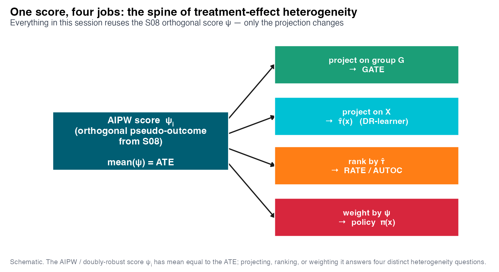
One object — the per-unit score \(\psi_i\) — powers everything today. Average it → ATE. Project / rank / weight it → GATE, \(\tau(x)\), RATE, policy.

This is the spine figure — keep coming back to it. The center is the AIPW pseudo-outcome psi_i from S08, the per-unit doubly-robust signal whose key property is that its conditional expectation IS the conditional effect: E[psi | X=x] = tau(x). Averaging it (the whole thing collapsed to one number) was last week. This week we do four other things with the same object. Each act lights up one arrow. Tell students that if they hold this picture, the methods stop looking like a zoo of unrelated estimators — GATE, DR-learner, RATE, and policy learning are four projections of one score.

When the Average Lies: Let the Effect Vary

On ShopSphere, the average effect is a trap

Symbol	ShopSphere	Role
\(D\)	coupon (0/1)	targeted discount
\(Y\)	profit_30d (€)	30-day profit
\(X\)	recency, frequency, monetary, tenure, age, channel, email opens, loyalty	customer covariates

A naive treated-minus-control difference says the coupon destroys profit: −€1.38. But the firm sends coupons to lapsing customers — who would have spent less anyway. The sign is confounded.

Meet the running example. ShopSphere is an online retailer; the marketing team sends a discount coupon (D) and measures 30-day profit (Y). The data are OBSERVATIONAL: the firm already targets coupons at lapsing and highly-engaged customers, so D is confounded by the same RFM covariates that drive profit. The naive treated-minus-control gap is MINUS 1.38 euros — the coupon looks actively harmful. That is pure confounding: coupon recipients are systematically different. This is exactly why we needed the S08 machinery — and it sets up the punchline that the average, once de-confounded, is small and positive, while the per-customer effect is wildly heterogeneous.

De-confounded, the average is real — but boring

Run the S08 AIPW estimator (cross-fitted \(\hat\mu_1,\hat\mu_0,\hat e\)) and the sign flips:

Estimator	Effect (€)	Verdict
Naive difference	−1.38	sign-flipped by confounding
Linear OLS (controls)	1.65	closer, still parametric
AIPW (DML)	≈ 1.5	CI covers truth (1.69)

So the coupon adds about €1.5 on average — “meh”. A blanket campaign barely breaks even. The average hides the action.

This is the de-confounding payoff and the motivation in one slide. The naive difference (−1.38) and the AIPW estimate (≈1.5, R gives 1.47, Python 1.52, CI covers the true ATE of 1.69) disagree even in SIGN — a dramatic Simpson-style reversal driven by targeting. Linear OLS with controls gets to 1.65, close, but we lean on the orthogonal AIPW number because it is the one whose per-unit pieces we will reuse. The verdict “meh on average” is the hook: an average effect of 1.5 euros makes the coupon look like a wash. The whole rest of the session shows that the average is the wrong summary — the effect ranges from strongly negative to strongly positive, and the money is in finding out for whom.

The object we want: the conditional effect \(\tau(x)\)

Define the conditional average treatment effect — the effect for customers like \(x\):

\[\tau(x) \;=\; \mathbb{E}\!\left[\,Y(1) - Y(0) \;\middle|\; X = x\,\right]\]

• ATE \(=\mathbb{E}[\tau(X)]\) — one number for the whole population (S08).
• CATE / IATE \(=\tau(x)\) — a function of the customer (today).
• GATE \(=\mathbb{E}[\tau(X)\mid G]\) — the effect for a named group (a coarsening of \(\tau(x)\)).

Same potential-outcome contrast as the ATE — just not averaged away. The ATE is \(\tau(x)\) collapsed to a point.

Define the central object cleanly. The CATE tau(x) is the expected treatment effect among units sharing covariate value x — the same potential-outcomes contrast Y(1)-Y(0) as the ATE, but conditioned on X instead of marginalized over it. Three estimands on one ladder of granularity: ATE (one number, the marginal mean of tau(X)); CATE / IATE (a full function of x — “individualized” though still an expectation over residual heterogeneity at x); GATE (the average of tau over a named, usually low-dimensional group G). The key conceptual point students must leave with: ATE = E[tau(X)], so the ATE is not a different thing — it is tau(x) integrated. Heterogeneity is what you see before you take that final average.

Heterogeneity needs no new identification

A natural worry: does conditioning on \(x\) require more assumptions? No.

By the law of iterated expectations, the ATE is just the average of the inner effects:

\[\text{ATE} \;=\; \mathbb{E}\big[\,\tau(X)\,\big] \;=\; \mathbb{E}\big[\,\mathbb{E}[Y(1)-Y(0)\mid X]\,\big]\]

If unconfoundedness \(\{Y(1),Y(0)\}\perp D \mid X\) identifies the outer average, it already identifies the inner effect \(\tau(x)\) — the same assumption, not yet averaged.

The reassurance

Heterogeneity is an estimation challenge (a function is harder than a number), not an identification one. The S08 assumptions carry over verbatim.

Address the assumption worry head-on because it is the most common confusion. Students assume that asking a harder question (a whole function instead of one number) must cost more assumptions. It does not. Unconfoundedness conditional on X identifies E[Y(1)-Y(0) | X=x] for every x — that conditional contrast is precisely tau(x). The ATE is then the iterated expectation over X. So identification of the CATE is FREE given S08’s selection-on-observables; what is hard is ESTIMATION: estimating a function well requires regularization, honesty, and validation, all of which can manufacture fake structure. The whole rest of the deck is about estimating and then validating tau(x), never about a new identification argument.

Two roles for a covariate: confounder vs effect-modifier

A variable in \(X\) can play two distinct roles — and they are independent:

Role	What it affects	If ignored…
Confounder \(C\)	both \(D\) and \(Y\)	bias — must adjust (identification)
Effect-modifier \(H\)	the size of \(\tau(x)\)	you miss heterogeneity (description)

A variable can be both, either, or neither. On ShopSphere frequency is both: it drives who gets a coupon (confounder) and how much the coupon helps (modifier).

Crucial: you condition on \(C\) to remove bias; you condition on \(H\) to describe variation. Different jobs, often the same columns.

This distinction prevents a lot of muddled thinking. A confounder C affects both treatment assignment and the outcome — you MUST adjust for it or your effect is biased; this is the identification job from S06-S08. An effect-modifier H changes the magnitude of the treatment effect — ignoring it does not bias the ATE, it just means you describe a single average where a richer picture exists; this is the description job of today. The two roles are logically independent: a variable can confound without modifying, modify without confounding, do both, or do neither. On ShopSphere frequency does both — the firm targets by frequency AND the coupon’s effect depends on frequency. The takeaway: adjusting for X buys identification; letting tau VARY with X buys understanding. Same X, two purposes.

IATE or GATE? A bias–variance choice

How finely should we resolve the effect? It is a bias–variance trade-off:

• IATE / \(\tau(x)\) — maximal resolution. Low bias, high variance: each \(x\) has little data, so individual estimates are noisy and hard to trust.
• GATE — coarse groups (e.g. frequency bands). Higher bias (averages within group), low variance: lots of data per cell, valid inference.

A useful division of labour

GATE is what you report (stable, interpretable, defensible SEs). \(\tau(x)\) is the engine that ranks and targets — even when no single \(\tau(\hat x)\) is individually precise.

Frame granularity as bias-variance. Going to the individual level minimizes bias (you condition on everything) but maximizes variance (almost no data at any single x), so individual estimates are too noisy to act on one at a time. Coarsening to groups injects bias (you average over within-group heterogeneity) but slashes variance and buys honest standard errors. The practical resolution — and a recurring theme — is a division of labour: report GATEs to stakeholders because they are stable and have defensible inference, but use the continuous tau(x) as the engine for ranking and targeting. You do not need each individual estimate to be precise for the RANKING to be useful, which is exactly what the validation and policy acts will exploit.

The score whose expectation IS the effect

Recall the S08 AIPW pseudo-outcome — the per-unit doubly-robust signal:

\[\psi_i = \big[\hat\mu_1(X_i) - \hat\mu_0(X_i)\big] + \frac{D_i\,(Y_i-\hat\mu_1(X_i))}{\hat e(X_i)} - \frac{(1-D_i)(Y_i-\hat\mu_0(X_i))}{1-\hat e(X_i)}\]

Its defining property — the spine of the whole session:

\[\boxed{\;\mathbb{E}\big[\psi \mid X = x\big] \;=\; \tau(x)\;}\]

So \(\psi_i\) is a noisy unbiased label for the unseen \(\tau(X_i)\). Averaging it gave the ATE; regressing it on \(X\) gives \(\tau(x)\). Every method today is a different regression of \(\psi\).

This is the load-bearing slide of the deck — the ψ-spine. The AIPW score from S08 is constructed so that its conditional expectation given X equals the conditional treatment effect: E[psi | X=x] = tau(x). That single identity is what licenses everything. It means psi_i is an unbiased (but noisy) LABEL for the latent tau(X_i) — we cannot observe Y(1)-Y(0) for any individual, but psi_i is a valid stand-in in conditional expectation. Therefore: averaging psi estimates E[tau(X)] = ATE (S08); regressing psi on a group indicator estimates the GATE (Act 2); regressing psi on X with a flexible learner estimates tau(x) (the DR-learner, Act 3); ranking by psi gives RATE (Act 4); weighting a classifier by psi gives the policy (Act 5). Hammer this: every method today is “regress the score on something.” This is the orthogonal score earning its keep beyond the ATE.

The roadmap: understand, validate, act

1. Understand — estimate \(\tau(x)\): GATE (Act 2), then causal forests & meta-learners (Act 3).
2. Validate — is the heterogeneity real? BLP test + RATE/TOC targeting curve (Act 4).
3. Act — turn \(\tau(x)\) into a deployable rule \(\pi(X)\): policy learning & policy trees (Act 5).

The discipline that makes this trustworthy: a flexible learner will always hand you a wiggly \(\hat\tau(x)\) — even from pure noise. Estimation is easy; earning belief in the estimate is the work.

Give students the map. Act 2 estimates the coarse, reportable version (GATE) directly from the score. Act 3 estimates the continuous engine tau(x) with forests and meta-learners. Act 4 is the conscience of the session: any sufficiently flexible model returns a varying tau-hat, so we MUST test whether the variation is real before we believe it — the BLP calibration test and the RATE/TOC targeting curve. Act 5 converts a validated tau(x) into an auditable decision rule. The warning at the bottom is the attitude to instill: producing a heterogeneous estimate is trivial and seductive; the professional skill is the validation step that separates signal from an overfit mirage.

Report the Group Effect: GATE from the Score

Stratify first — the honest, coarse view

The simplest heterogeneity analysis: split customers into pre-specified groups and estimate the effect within each.

• Pick a small number of policy-relevant groups (frequency bands, channels, loyalty tiers).
• Estimate the effect in each cell with a valid ATE estimator (e.g. AIPW per group).

Two rules for honest stratification

Coarse: few groups, chosen before seeing outcomes — not data-dredged. Pre-specified: subgroups picked after looking at \(\hat\tau\) are how false discoveries are born.

Stratification is the oldest heterogeneity tool and still the right first move when groups are known in advance. Define a handful of policy-relevant cells — here frequency bands — and estimate a clean, identified effect inside each, ideally with the same AIPW machinery so each cell-level number is de-confounded. The two discipline rules matter: keep the groups COARSE (few cells, so each has data and valid inference) and PRE-SPECIFY them before peeking at outcomes. The classic sin is to slice every which way, find a subgroup with a big effect, and report it — that is multiple testing in disguise and a reliable source of effects that vanish on replication. Pre-registration of subgroups is the antidote.

The interaction trap: a confounded coefficient

Tempting shortcut: one OLS with a treatment × modifier interaction — \[Y = \alpha + \tau\,D + \gamma\,H + \delta\,(D\times H) + \varepsilon\] and read \(\delta\) as “how the effect varies with \(H\)”.

Why this breaks

If \(H\) is also a confounder, the interaction \(\delta\) is biased by the same confounding that biases \(\tau\) — and the controls enter linearly, so any nonlinear confounding leaks straight into \(\hat\delta\).

On ShopSphere frequency confounds and modifies — exactly the case where the raw interaction misleads. We need a method that de-confounds first, then describes variation.

This is the trap that makes naive heterogeneity analysis dangerous. Throwing a D×H interaction into OLS feels like the obvious move, but the interaction coefficient inherits all the confounding pathologies of the main effect: if H drives selection into treatment, delta is biased, and because OLS adjusts linearly, any nonlinear confounding contaminates both tau and delta. On ShopSphere frequency is simultaneously a confounder and a modifier — the worst case — so the raw interaction conflates “the coupon helps frequent buyers more” with “frequent buyers were targeted and differ anyway.” The fix is to separate the two jobs: de-confound with the orthogonal score FIRST, then describe how the de-confounded effect varies. That is exactly what regressing psi on the group does.

GATE = regress the score on the group

The spine, second appearance. We already have a de-confounded per-unit label \(\psi_i\) with \(\mathbb{E}[\psi\mid X]=\tau(x)\). So regress \(\psi\) on group dummies:

\[\widehat{\text{GATE}}(g) \;=\; \frac{1}{n_g}\sum_{i \,\in\, g} \psi_i \;=\; \bar\psi_{\,g}\]

That is just the group mean of the score — and an OLS of \(\psi\) on group indicators returns each GATE as a coefficient with a valid standard error.

The confounding was already removed when we built \(\psi\) (cross-fitted \(\hat\mu_1,\hat\mu_0,\hat e\)). No interaction trap: de-confound first (in \(\psi\)), then describe (by group).

Here is the clean alternative to the interaction trap, and the second appearance of the spine. Because psi already has the confounding removed — it was built from cross-fitted outcome and propensity models — its conditional mean is tau(x). So the GATE for group g is simply the average of psi over that group’s members, and operationally you run an OLS (or doubleml’s group-ATE routine) of psi on group dummies; each coefficient is a GATE and comes with a standard error. The contrast with the previous slide is the whole point: the interaction approach de-confounds and describes in ONE linear model and gets both wrong; the score approach de-confounds flexibly when building psi, then describes with a trivial group mean. Order of operations is everything.

Why the inference is valid

Two reasons the GATE standard errors are trustworthy:

• The score is orthogonal. Small errors in the nuisances \(\hat\mu_1,\hat\mu_0,\hat e\) do not contaminate \(\bar\psi_g\) to first order — the same Neyman orthogonality that made the S08 ATE valid.
• The groups are pre-specified and low-dimensional. A handful of fixed cells means standard OLS inference on \(\psi\) applies directly — no post-selection penalty. (Semenova and Chernozhukov 2021)

The free lunch

Group-level heterogeneity comes with honest confidence intervals — because it is just an average of an orthogonal score over fixed groups.

Explain why GATE inference is genuinely valid, not just convenient. First, orthogonality: psi is the Neyman-orthogonal AIPW score, so its group average is insensitive to first-order nuisance error — the same property that gave the ATE a trustworthy interval transfers to every group mean. Second, the groups are fixed in advance and few, so we are doing ordinary inference on a pre-specified low-dimensional summary; there is no data-driven subgroup selection to correct for. Semenova and Chernozhukov formalize this for group and best-linear-projection summaries of the CATE. The headline: GATEs are the one heterogeneity object you get with honest confidence intervals essentially for free — which is exactly why they are what you report to decision-makers.

The coupon helps the lapsed — and hurts the loyal

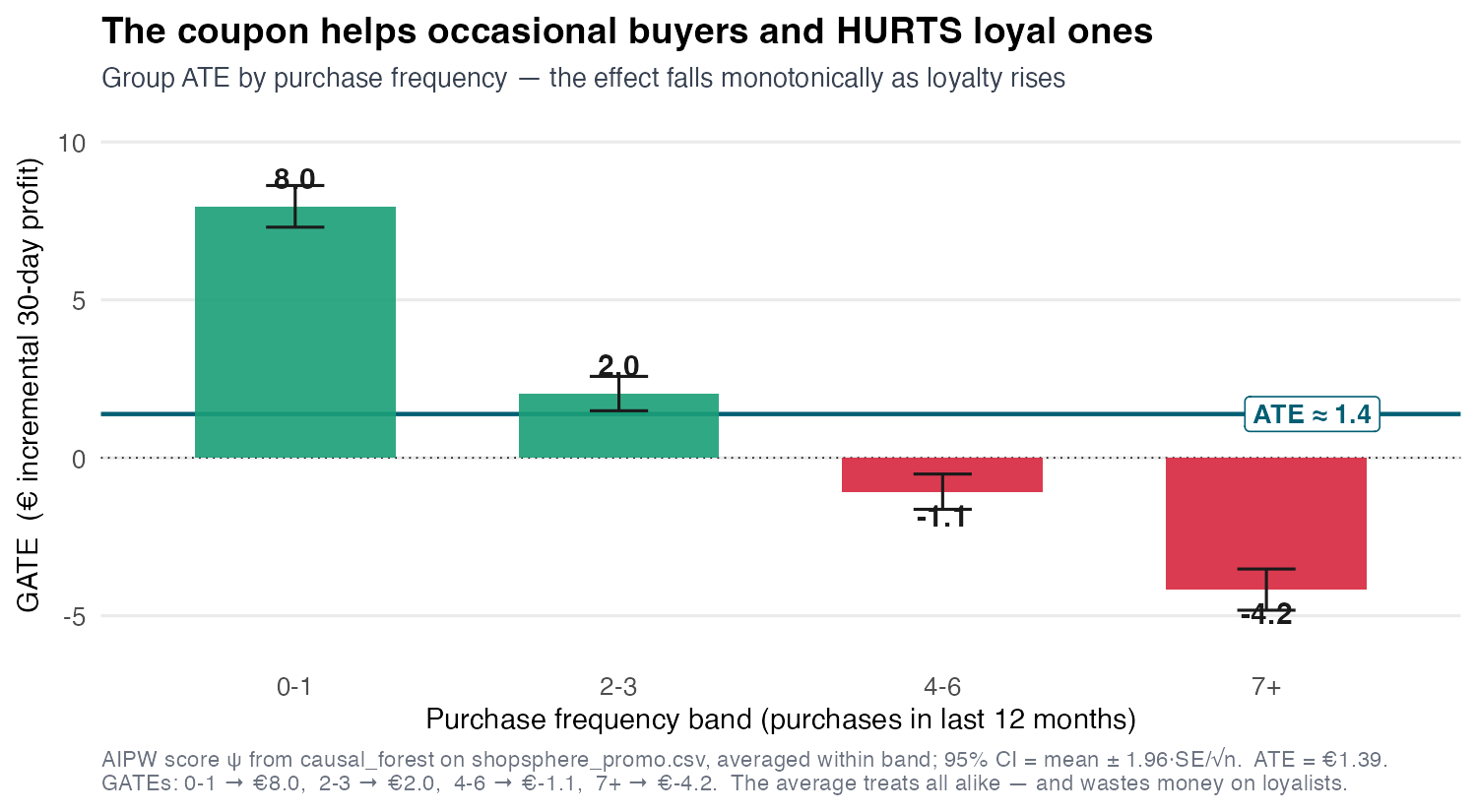
GATE by frequency band: 0–1 buys: +€8.0 · 2–3: +€2.0 · 4–6: −€1.1 · 7+ buys: −€4.2. The “meh” €1.4 average was masking a sign change.

This figure is the emotional core of the session. The de-confounded GATE by purchase-frequency band moves monotonically from strongly positive for lapsing customers (0-1 prior purchases: +8.0 euros) down through near-zero to clearly negative for the most loyal (7+ purchases: -4.2 euros). The 1.4-euro average was the meaningless midpoint of a distribution that ranges from +8 to -4. Business reading: coupons reactivate lapsing customers (persuadables) but cannibalize margin on loyal customers who would have bought at full price (the “sure things” / “do-not-disturb” cell). This is the whole argument for targeting in one chart — and it is the coarse, reportable GATE view. The continuous engine that lets us target individuals, not just bands, comes next.

From bands to a smooth curve

Bands are reportable but blunt. To resolve \(\tau\) along a continuous modifier, replace group dummies with a flexible basis:

\[\widehat{\tau}(h) \;=\; \text{smooth of } \psi_i \text{ on } h_i \qquad (\text{kernel or spline regression of the score})\]

Same spine — regress \(\psi\) on the modifier — but the “groups” become a continuum. This recovers a curve instead of bars.

But once the modifier is multivariate (frequency and recency and tenure …), hand-picked bases break down. We need a learner that finds the structure itself — Act 3.

Bridge from groups to the continuous engine in one line, kept deliberately light per the altitude decision. Replacing group dummies with a kernel or spline basis turns the bar chart into a smooth tau(h) along a single continuous modifier — still the spine, still “regress psi on the modifier,” just with a richer basis. This is fine for one or two pre-chosen modifiers. It collapses when heterogeneity lives in many covariates and unknown interactions, because you cannot hand-specify the basis. That motivates Act 3: instead of choosing the basis, let a forest or a meta-learner discover where tau varies. Mention but do not dwell — GATES and series estimators live in the notes.

GATE reports, \(\tau(x)\) targets

The division of labour, restated

GATE — coarse, honest CIs, board-ready. The number you put in a slide deck for stakeholders. \(\tau(x)\) — fine, individual-level, the engine that drives ranking and targeting.

You can report GATEs and still act on \(\tau(x)\) — the two are complementary, not competing.

Next: estimate the continuous \(\tau(x)\) — and confront the fact that flexible learners invent heterogeneity if you let them.

Consolidate Act 2 before moving up in resolution. The GATE is the communication layer: coarse, interpretable, with defensible confidence intervals — what you actually present to a marketing director. The continuous tau(x) is the decision layer: it drives the ranking and the targeting rule even if no single point estimate is individually precise. These are complementary roles for the same underlying object, not rival estimators. The cliffhanger for Act 3 is the central danger of continuous estimation: a flexible learner will ALWAYS return a wiggly tau-hat(x), whether or not real heterogeneity exists — so Act 3 builds the estimators and Act 4 builds the lie-detector.

Estimating the Engine: Forests & Meta-Learners

The obvious idea: model each arm, subtract

The meta-learner recipe: build \(\tau(x)\) out of off-the-shelf regressions.

• S-learner (single): fit one model \(\hat\mu(D,X)\) with \(D\) as a feature; \(\hat\tau(x)=\hat\mu(1,x)-\hat\mu(0,x)\).
• T-learner (two): fit \(\hat\mu_1(x)\) on the treated and \(\hat\mu_0(x)\) on the controls separately; subtract.

Both are intuitive and use any regressor you like. But both optimize the wrong objective — next slide.

Start meta-learners with the two most intuitive. The S-learner fits a single outcome model with treatment as just another feature and differences the two predictions; its weakness is that regularization can shrink the treatment feature toward irrelevance, washing out the effect. The T-learner fits two completely separate models, one per arm, and subtracts; it avoids shrinking away D but wastes data (each model sees only half the sample) and the two models can have very different smoothness, injecting spurious structure into the difference. Both are appealing because they reuse any regressor. The conceptual problem they share — they optimize prediction of Y, not estimation of tau — is the subject of the next slide and the reason causal-specific methods exist.

Predicting \(Y\) well ≠ estimating \(\tau\) well

The meta-learner critique

S- and T-learners minimize outcome prediction error (MSE on \(Y\)). But \(\tau(x)\) is a difference of two large surfaces — a learner tuned to predict \(Y\) can be badly tuned to estimate their difference. (Curth and Schaar 2023)

Two failure modes:

• S-learner: regularization can shrink the weak \(D\) signal toward zero — understating heterogeneity.
• T-learner: two independently-tuned models differ in smoothness; their difference inherits spurious structure.

The cure: target the causal quantity directly — split on effect heterogeneity (forests) or regress the score (DR-learner). (Lechner 2018)

This is the conceptual hinge of Act 3 — say it slowly. Off-the-shelf learners are trained to minimize prediction error on Y. But the object we want, tau(x) = mu1(x) - mu0(x), is a DIFFERENCE of two surfaces, and a model that predicts each surface well can estimate their difference poorly — small correlated errors in mu1 and mu0 can swamp the true gap. Two concrete failure modes: the S-learner’s regularization can shrink the treatment signal so heterogeneity is understated; the T-learner’s two models have independent bias-variance trade-offs, so their difference carries structure that is an artifact of differential smoothing, not real heterogeneity. Lechner calls this the joint-goal / mean-squared-causal-error problem. The fix that defines the rest of the act: optimize for the causal target directly — causal forests split on effect difference, the DR-learner regresses the orthogonal score.

Causal trees: split where the effect differs

A causal tree changes the splitting rule. A regression tree splits to make \(Y\) homogeneous; a causal tree splits to make the treatment effect differ across leaves.

• Each leaf is a subgroup; the leaf’s effect estimate is the within-leaf treated-minus-control gap.
• Splits are chosen to maximize the difference in \(\hat\tau\) between child leaves.

The danger: choosing and estimating on the same data

Pick the split and estimate the leaf effect from the same rows, and you bias the effect toward the split — the leaf looks more extreme than it is. (Overfitting the heterogeneity.)

Causal trees, the building block of forests, in intuition only per the altitude decision. The single idea: change what the tree optimizes. A standard CART splits to reduce variance in Y; a causal tree (Athey-Imbens) splits to MAXIMIZE the difference in estimated treatment effect between the resulting leaves, so the partition tracks effect heterogeneity rather than outcome level. The leaf effect is the within-leaf treated-minus-control contrast. The catch, which motivates the next slide: if you use the same observations to choose the splits AND to estimate the leaf effects, you get adaptive overfitting — the splitting search finds the rows where the effect looks biggest, so the leaf estimates are exaggerated in the direction of the split. We do NOT derive the splitting criterion; that is in the notes.

Honesty: separate the splitting from the estimating

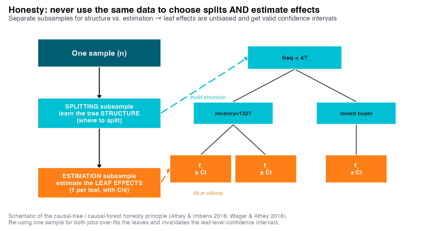
Honest estimation: use one subsample to choose the splits, a different subsample to estimate the leaf effects. The effect estimate never sees the data that chose its split → unbiased within-leaf. (Athey and Imbens 2016)

Honesty is Athey and Imbens’s fix for the adaptive-overfitting problem, and it is the conceptual ancestor of cross-fitting from S08 — same logic, different setting. Partition the training data into two disjoint subsamples: one grows the tree (decides where to split), the other estimates the effect inside each leaf. Because the leaf estimates are computed on rows that played no part in choosing the partition, they are unbiased for the within-leaf effect and come with valid confidence intervals. The cost is statistical efficiency — you spend half your data on structure and half on estimation — but the payoff is honest inference. This is the same don’t-let-a-unit-be-predicted-by-a-model-that-was-trained-on-it discipline as cross-fitting, applied to tree leaves.

Causal forests: many honest trees, adaptively weighted

A causal forest averages many honest causal trees — but it is more than an average. (Wager and Athey 2018; Athey, Tibshirani, and Wager 2019)

• Each tree defines, for a target point \(x\), which training units fall in its leaf — i.e. which units are “like \(x\)”.
• Across trees, this yields adaptive weights \(\alpha_i(x)\): data-driven neighbours of \(x\), with the forest deciding which covariates matter for similarity.
• \(\hat\tau(x)\) solves a local estimating equation, weighting units by \(\alpha_i(x)\).

In effect: a forest is adaptive nearest-neighbour matching, where the metric is learned to track effect heterogeneity — not outcome level.

Causal forests at the right altitude — intuition, no influence-function or alpha-weight algebra (that is in the notes). The key reframe, due to Wager-Athey and the generalized-random-forest paper: a forest is not really an ensemble of predictions, it is a way to LEARN a similarity weighting. For any target x, each honest tree says which training units share x’s leaf; aggregating over trees gives smooth adaptive weights alpha_i(x) that define x’s effective neighbours. The forest then solves a LOCAL moment equation at x, weighting units by alpha_i(x). The one-sentence intuition students should keep: a causal forest is adaptive nearest-neighbour matching where the distance metric is learned from the data to emphasize the covariates that drive effect heterogeneity, not the ones that drive the outcome level. That learned metric is exactly what fixes the S/T-learner critique.

The forest solves a locally-weighted version of the same moment

At each target point \(x\), the forest estimates \(\hat\tau(x)\) by solving a locally-weighted version of the same moment we have used all along — units near \(x\) count more:

\[\sum_i \alpha_i(x)\,\psi\big(W_i;\,\tau(x)\big) \;=\; 0\]

• \(\alpha_i(x)\) — the forest’s learned similarity weights (how much unit \(i\) looks like \(x\)).
• \(\psi\) — the same orthogonal score from S08, on unit \(i\)’s data \(W_i=(Y_i, D_i, X_i)\).

So the forest is the local cousin of DML: globally average the score → ATE; locally weight it → \(\tau(x)\). (Splitting algebra lives in the notes.)

State — do not derive — what the forest computes. It solves a locally-weighted moment condition: the same orthogonal score psi we have used since S08, summed with the forest’s learned weights alpha_i(x) and set to zero, gives tau-hat(x). Read against the spine: DML set the UNWEIGHTED average of the score to zero to get the ATE; the causal forest sets a LOCALLY-WEIGHTED average to zero to get tau(x). Same score, same orthogonality (so the local estimate inherits robustness to nuisance error), just neighbourhood weights instead of uniform ones. This is the cleanest way to see forests and DML as one family. The actual gradient-based splitting rule and the influence-function expression for alpha are deferred to the notes per the calibrated-triage altitude.

The forest recovers the true effect; the T-learner is noisier

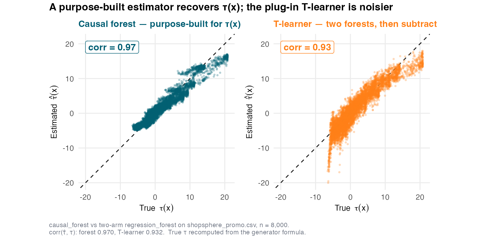
Estimated vs known true \(\tau(x)\): causal forest tracks truth at corr 0.97; the T-learner is visibly noisier at corr 0.93. Targeting the causal quantity pays off.

The recovery plot validates the whole apparatus because ShopSphere is simulated — we KNOW the true tau(x), so we can plot estimate against truth. The causal forest hugs the 45-degree line with correlation 0.97 (R 0.970, Python 0.967); the T-learner, which optimizes outcome prediction rather than the causal target, is visibly more scattered at 0.93 (R 0.932; Python’s T-learner is noisier still at 0.879, and the DR-learner around 0.81 — an estimator-and-defaults gap we document in the lab, not force-match). The lesson lands the S/T critique empirically: methods that target the difference directly recover heterogeneity better than methods that target the outcome and subtract. With real data you never get this plot — which is precisely why Act 4’s validation tools exist.

See the heterogeneity: a wide spread of effects

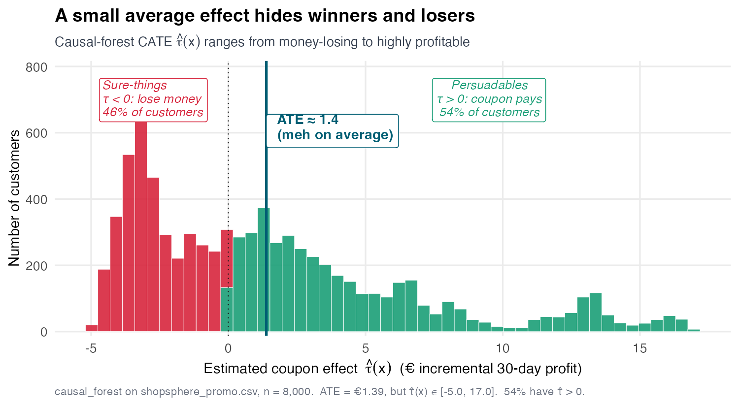
The estimated \(\hat\tau(x)\) ranges from −€5 to +€17 (SD ≈ 5.0), centred near the €1.4 ATE. About 54% of customers have a positive estimated effect. The average was the tip of an iceberg.

This histogram is the punchline of the understand phase. The distribution of the forest’s estimated individual effects is wide — standard deviation about 5 euros — ranging from roughly -5 (the coupon clearly destroys margin) to +17 (the coupon is enormously profitable), with the mass centred near the 1.4-euro forest ATE and about 54% of customers above zero. (The TRUE effects are wider still, spanning -6.5 to +20.8 with 51.5% positive — the recovery slide compares estimate against truth; the forest compresses the spread slightly, as flexible learners do.) The ATE was a thin slice through a fat distribution. Business implication: roughly half the customer base should never get the coupon, and a minority is wildly profitable to target — exactly the structure that makes a targeting policy worth far more than treat-everyone. But remember Act 4’s warning: a flexible learner can DRAW a wide histogram even from noise, so this picture is a hypothesis to be tested, not yet a finding.

A field guide to meta-learners: what each regresses

Learner	What it regresses	Targets \(\tau\) directly?	Watch out for
S	\(Y\) on \((D,X)\), one model	no (difference of preds)	shrinks \(D\) away
T	\(Y\) on \(X\) per arm, two models	no (difference of preds)	mismatched smoothness; halves data
X	imputed unit effects on \(X\), propensity-blended	closer	helps under treatment imbalance
R	\(\tilde Y\) on \(\tilde D\) (Robinson residuals), \(\tau(x)\)-weighted	yes	needs good nuisances
DR	the AIPW score \(\psi\) on \(X\)	yes (orthogonal)	the spine — our default

The pattern: S/T predict \(Y\) and subtract; X/R/DR target \(\tau\) itself. Causal forests can fit the R- or DR-style objective internally. (Künzel et al. 2019; Nie and Wager 2021; Kennedy 2023)

This table is the consolidating artifact of Act 3 — organize it by “what each learner regresses,” not by name. S and T regress the OUTCOME and subtract predictions (indirect, the critique applies). X-learner imputes individual effects and blends the two arms by the propensity, which helps a lot when one arm is much smaller (treatment imbalance) — Künzel et al.’s motivation. R-learner regresses the Robinson residual of Y on the residual of D, weighting by the local effect, so it targets tau directly (Nie-Wager). DR-learner regresses the AIPW score psi on X — the spine, third appearance — and is orthogonal, which is why it is our default (Kennedy). The unifying sentence students should memorize: S/T predict Y and subtract; X/R/DR go after tau itself. Causal forests can be cast as fitting the R- or DR-objective internally, which is why grf and the DR-learner agree closely on ShopSphere.

X-learner: borrow strength under imbalance

When one arm is much larger (few treated, many controls — common in observational data), the X-learner uses both arms efficiently: (Künzel et al. 2019)

1. Fit \(\hat\mu_1,\hat\mu_0\) (the T-learner step).
2. Impute each unit’s effect using the other arm’s model: \(\hat\tau_i = Y_i - \hat\mu_0(X_i)\) for treated, \(\hat\mu_1(X_i) - Y_i\) for controls.
3. Regress these on \(X\) within each arm → \(\hat\tau_1\) (treated), \(\hat\tau_0\) (control), then blend by the propensity:

\[\hat\tau(x)\;=\;\big(1-\hat e(x)\big)\,\hat\tau_1(x)\;+\;\hat e(x)\,\hat\tau_0(x)\]

The blend leans on the larger arm’s (better-estimated) model where data is thin — visibly better than the plain T-learner when treatment is rare.

The X-learner gets one slide because its specific virtue — imbalance — is common in observational marketing data where few customers are treated. Step 1 is the T-learner. Step 2 is the clever bit: impute a pseudo-effect for every unit using the OTHER arm’s model (a treated unit’s effect is its outcome minus what the control model predicts for it, and vice versa). Step 3 smooths those imputed effects over X within each arm and blends the two estimates with the propensity as the weight: \(\hat\tau(x)=(1-\hat e)\,\hat\tau_1+\hat e\,\hat\tau_0\). Note the direction — the treated-arm estimate \(\hat\tau_1\) leans on the plentiful controls’ model \(\hat\mu_0\), so it gets the large weight \(1-\hat e\) exactly when treatment is rare; the better-estimated (larger) arm dominates where the smaller arm is data-starved. The result is markedly more stable than the T-learner when treatment is rare. On ShopSphere treatment is balanced (50%), so X-learner gains little here, but name the use case so students reach for it correctly.

R-learner: the Robinson residual, made local

The R-learner targets \(\tau(x)\) through the Robinson partialling-out you know from DML — now with a slope that varies in \(x\): (Nie and Wager 2021)

\[\hat\tau(\cdot) \;=\; \arg\min_{\tau}\ \sum_i \Big[\underbrace{(Y_i-\hat\ell(X_i))}_{\tilde Y_i} - \tau(X_i)\,\underbrace{(D_i-\hat e(X_i))}_{\tilde D_i}\Big]^2\]

\(\hat\ell(X)=\mathbb{E}[Y\mid X]\), \(\hat e(X)=\mathbb{E}[D\mid X]\) are the S08 cross-fitted nuisances; built on \(\tilde Y,\tilde D\) it inherits DML’s orthogonality.

Factor out \(\tilde D_i^2\) → an ordinary weighted regression:

\[\hat\tau(\cdot) \;=\; \arg\min_{\tau}\ \sum_i \underbrace{(D_i-\hat e(X_i))^2}_{\text{weight } w_i}\,\Big(\underbrace{\tfrac{Y_i-\hat\ell(X_i)}{D_i-\hat e(X_i)}}_{\text{pseudo-outcome } \tilde Z_i}\;-\;\tau(X_i)\Big)^2\]

Regress \(\tilde Z_i=\tilde Y_i/\tilde D_i\) on \(X\), weighted by \(w_i\) — any sample-weight learner (forest, boosting, NN) fits it; the weight vanishes where \(\tilde D_i\to0\), so \(\tilde Z_i\) can’t explode.

The slide now carries BOTH forms: the linear/Robinson residual-on-residual objective AND its generic-ML reformulation. Students already met Robinson partialling-out in S08 — residualize Y and D on X, regress residual on residual, read the slope as the ATE. The R-learner is exactly that with one change: the slope tau is allowed to vary with x rather than be a constant.

The reveal is one line of algebra. Factor the squared treatment residual out of the bracket: [Ytilde - tau*Dtilde]^2 = Dtilde^2 * (Ytilde/Dtilde - tau)^2. The objective is now an ORDINARY WEIGHTED LEAST SQUARES — regress the pseudo-outcome Ztilde = Ytilde/Dtilde on X, with weights w = Dtilde^2 = (D - ehat)^2. THAT is what “generic ML” means here: any supervised learner that accepts sample weights (random forest, gradient boosting, a neural net) minimizes this loss — no bespoke solver needed.

The weighting is also what keeps the pseudo-outcome numerically sane: units with a strong treatment signal (large |Dtilde|) get the most weight, while units with Dtilde near zero — exactly where the ratio Ytilde/Dtilde would blow up — are down-weighted toward zero, so the explosion is harmless. Built on the orthogonalized residuals, it inherits Neyman orthogonality and robustness to small nuisance error. One-line takeaway: “Robinson with a varying slope, fit as a weighted regression of a pseudo-outcome” (Nie & Wager 2021). The matching derivation is in the notes, sec-metalearners.

DR-learner: regress the score on \(X\) — the spine, again

The third appearance of the spine — and our default. Take the per-unit AIPW score and regress it on the covariates: (Kennedy 2023)

\[\hat\tau(x) \;=\; \widehat{\mathbb{E}}\big[\,\psi \,\big|\, X = x\,\big], \qquad \mathbb{E}[\psi\mid X=x]=\tau(x)\]

• Stage 1: cross-fit the nuisances \(\hat\mu_1,\hat\mu_0,\hat e\) → build \(\psi_i\) (S08).
• Stage 2: regress \(\psi_i\) on \(X\) with any flexible learner.

Doubly robust and orthogonal, so the second-stage learner can be a black box without contaminating \(\tau(x)\) to first order. This is why a causal forest fit on \(\psi\) recovers truth so well.

The DR-learner is the cleanest expression of the spine and the deck’s recommended default. Two stages: first, cross-fit the outcome and propensity nuisances and assemble the AIPW pseudo-outcome psi_i exactly as in S08; second, regress psi on X with any flexible learner — because E[psi|X]=tau(x), that regression IS the CATE estimate. Kennedy’s result is that this is doubly robust and orthogonal, so the second-stage learner can be arbitrary (a forest, gradient boosting, a neural net) without first-order contamination from nuisance error. This is the third explicit reuse of psi — averaged=ATE, grouped=GATE, now regressed on X=tau(x) — and it explains why the grf forest and the DR-learner give nearly identical, high-correlation recovery on ShopSphere: they are fitting essentially the same orthogonal target.

Which learner? None dominates — match the problem

Practical guidance

Default to DR-learner / causal forest (orthogonal, targets \(\tau\)). Reach for the X-learner under heavy treatment imbalance. Use S/T only as quick baselines. (Curth and Schaar 2023)

But there is no universally best learner — the winner depends on the true \(\tau(x)\) surface (smooth vs sparse vs sharp), the sample size, and overlap.

The unifying lesson

What makes all the good ones good is the same thing: an orthogonal score that targets \(\tau\) directly, not the outcome \(Y\).

Set realistic expectations. The honest empirical finding from the meta-learning literature (Curth and van der Schaar) is that NO single learner wins across data-generating processes — performance depends on the shape of the true CATE surface, sample size, and overlap. So the guidance is a decision rule, not a ranking: default to the orthogonal, tau-targeting methods (DR-learner or causal forest); switch to the X-learner when treatment is rare; keep S/T as fast sanity baselines. The deeper unifying point ties the whole act together: the methods that work share one ingredient — an orthogonal score aimed at tau rather than at predicting Y. That is the same Neyman orthogonality from S08, now doing heterogeneity duty. Which is the perfect cue for Act 4: orthogonality makes the estimate well-behaved, but it does not tell you whether the heterogeneity is REAL.

The orthogonal score does the heavy lifting

Step back. Across forests, R-learner, and DR-learner, the engine is the same:

• Partial \(X\) out of \(Y\) and \(D\) (cross-fitted nuisances) — the S08 move.
• Target \(\tau\) directly via an orthogonal score, locally (forest weights) or by regression (DR-learner).
• Inherit robustness: small nuisance errors do not contaminate \(\hat\tau(x)\) to first order.

So heterogeneity estimation is not a new paradigm — it is DML, refusing to take the final average.

Close Act 3 by collapsing the zoo back to one idea. Every good CATE estimator does the same three things: partials X out of Y and D with cross-fitted nuisances, targets tau directly through an orthogonal score (the forest does it with local weights, the DR-learner with a second-stage regression), and inherits first-order robustness to nuisance error. The slogan to leave on screen: heterogeneity is DML refusing to take the final average. That sentence connects S08 and S09 into one method and sets up the pivot — we can now estimate tau(x) reliably, but estimation reliability is not the same as the heterogeneity being real. Act 4 is the lie-detector.

Is the Heterogeneity Real? Validation

A flexible learner always draws a wiggle

The uncomfortable truth

Fit a causal forest on data with zero true heterogeneity (\(\tau(x)\equiv\text{const}\)) and you still get a varying \(\hat\tau(x)\) — a wiggly histogram of pure noise.

The estimate looks the same whether heterogeneity is real or invented. So before acting, we must answer two questions with inference, not eyeballing:

1. Is it real? Does \(\hat\tau(x)\) carry genuine signal about the true effect? → BLP / calibration test
2. Is it worth it? Would targeting by \(\hat\tau(x)\) actually beat treating everyone? → RATE / TOC

Open the validation act with the failure mode it exists to catch. A flexible learner has the capacity to fit noise, so running it on a constant-effect DGP still yields a varying tau-hat and a wide histogram — visually indistinguishable from the real thing. You therefore cannot trust your eyes; you need formal tests. Two distinct questions, two distinct tools. Is it real: does the estimated CATE actually carry information about the true effect, or is it noise dressed as structure — answered by the best-linear-projection / calibration test. Is it worth it: even if real, does targeting by tau-hat beat a blanket policy by enough to matter — answered by the RATE and the targeting operator characteristic (TOC) curve. Both are the spine again: tests built on the score.

The BLP test: does \(\hat\tau(x)\) predict the true effect?

Regress the orthogonal score \(\psi\) on the (out-of-fold) estimate \(\hat\tau(x)\) — the spine doing validation:

\[\psi_i \;=\; \beta_1 + \beta_2\,\big(\hat\tau(X_i) - \overline{\hat\tau}\big) + \varepsilon_i\]

• \(\beta_1\) — calibration of the level: is the average effect right? (≈ ATE.)
• \(\beta_2\) — calibration of the slope: when \(\hat\tau\) says “bigger”, is the effect actually bigger?

The decisive coefficient

\(\beta_2 = 1\): \(\hat\tau\) is perfectly calibrated. \(\beta_2 = 0\): \(\hat\tau\) is noise — it does not track the truth. Test \(H_0\!:\beta_2=0\). (Chernozhukov et al. 2018)

The best-linear-projection / calibration test is the lie-detector, and it is once again the spine — regress the orthogonal score psi on the estimated CATE. Two coefficients with clean interpretations. Beta_1 is the level calibration: the intercept recovers the average effect, sanity-checking against the ATE. Beta_2 is the slope calibration and the one that matters: it asks whether, when your model says the effect is larger, the de-confounded score actually IS larger. If beta_2 = 1 the estimate is perfectly calibrated; if beta_2 = 0 the estimate is pure noise with no relation to the truth. The formal test is H0: beta_2 = 0 — reject it and you have evidence of real, correctly-ordered heterogeneity. Chernozhukov et al.’s generic-ML framework formalizes this (and the BLP A/B strategies, which live in the notes per the altitude call).

On ShopSphere, the heterogeneity is unmistakably real

Quantity	Estimate	Reading
Is the ranking real?  test_calibration(cf) — project the score on the forest’s own \(\hat\tau\)
Differential prediction (\(\beta_2\))	1.08  (\(t = 36.6\))	\(\hat\tau\) tracks truth, slope ≈ 1
Mean-forest calibration (\(\beta_1\))	0.955	level ≈ correct (ATE)
What drives it?  best_linear_projection(cf, ·) — project on named covariates
Slope on frequency	−1.19  (\(p<2\!\times\!10^{-16}\))	effect falls as frequency rises

\(\beta_2 = 1.08\), \(p < 2\times10^{-16}\): we decisively reject \(H_0\!:\beta_2=0\) — the wide histogram was signal, not noise. A separate projection onto covariates then pins the gradient — the effect falls €1.19 per purchase — confirming the negative driver the GATE bars already ranked dominant.

TWO different projections of the same orthogonal score — say so explicitly, because the slide lists both. FIRST, the calibration test (grf’s test_calibration): regress psi on the forest’s OWN prediction tau-hat. The differential-prediction coefficient beta_2 = 1.08, t = 36.6 — slope essentially 1, so the forest’s ordering of customers matches the true ordering almost perfectly; reject the no-heterogeneity null at p < 2e-16. beta_1 = 0.955 says the level is right too (recovers the ATE). SECOND, a SEPARATE call (best_linear_projection on named covariates): the score projected on frequency gives -1.19, p < 2e-16 — the effect declines as purchase frequency rises. Stress that this second number is a GRADIENT, not a dominance test: ‘dominant’ is the GATE bars’ verdict from Act 2 (and the standardized comparison — frequency about -4 per SD versus recency -2), which this slope corroborates in direction. (Python’s manual beta_2 is 1.30, t = 43.8 — same conclusion, different scaling; we report grf’s calibrated version.) Conclusion: the heterogeneity is real (the calibration test) and we can read its main driver’s gradient (the covariate projection). Now: is it worth acting on?

Is it worth it? RATE ranks, then measures the gain

Real heterogeneity is necessary but not sufficient — we need to know targeting pays. The RATE (Rank-Weighted Average Treatment Effect) measures the gain from prioritizing by \(\hat\tau\): (Yadlowsky et al. 2025)

• Rank customers by \(\hat\tau(x)\), high to low (the spine: rank by the score).
• Treat the top \(q\) fraction; compute how much more effect they get than treating everyone — their average effect minus the overall ATE.
• Plot that benefit-over-treat-all against \(q\) → the TOC (Targeting Operator Characteristic) curve (it decays to 0 at \(q=1\)).

RATE = area under the TOC

If \(\hat\tau\) ranks well, the top customers gain much more than treating everyone — the TOC stays above the flat random-targeting line at 0. RATE > 0 (a QINI cousin) certifies the ranking has value.

RATE answers the worth-it question and is the spine in its ranking guise (Yadlowsky et al., now in JASA). The recipe: rank customers by their estimated CATE, sweep a treatment fraction q from 0 to 1, and at each q record how much more effect the top-q customers get than treating everyone — their average effect minus the overall ATE (the benefit over treat-all). Plot it: that is the TOC curve, which decays to 0 at q = 1. If the ranking is informative, the top-ranked customers benefit far more than average, so the curve starts high (~€12 of benefit over treat-all for the top few percent) and decays to 0 — the area between the curve and the flat random-targeting line at 0 is the RATE. A positive RATE certifies that prioritizing by tau-hat beats random/blanket treatment; it is the heterogeneity cousin of the Qini/uplift curve from marketing. Note RATE measures the VALUE of the ranking, complementing BLP which measures whether the ranking is correct — you want both.

The targeting curve: front-loaded gains

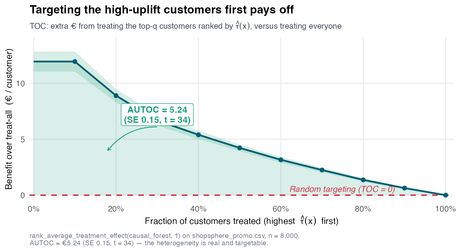
\(\widehat{\mathrm{TOC}}(q)=\overline{\psi}\,\big|_{\text{top-}q\text{ by }\hat\tau}-\overline{\psi}_{\text{all}}\)  —  the benefit over treat-all, scored by the doubly-robust \(\psi\) (rank by \(\hat\tau\), score by \(\psi\))

Treat the top-ranked customers and you gain far more than treating everyone — about €12/customer extra for the top decile, shrinking to €0 once you treat the whole base. RATE (AUTOC) = 5.24 (\(t = 34\)) — the ranking has real, sizeable value.

Read the TOC. The y-axis is the extra euros per customer over treating everyone (the top-q average effect minus the overall ATE); the x-axis is how many you treat. The curve is steeply front-loaded: the highest-ranked few percent show ~€12 of benefit over treat-all, and as you extend treatment down the ranking that benefit erodes to 0 — exactly the signature of a valuable ranking. The area between the curve and the flat random-targeting line at 0 is the AUTOC-style RATE = 5.24 with a standard error of 0.15 (t = 34), decisively positive. (Python’s manual RATE is 6.35 — estimator-and-scale differences we document rather than force-match, same family as S08’s reported parity gaps.) Together with the BLP test, we now have both certificates: the heterogeneity is real (BLP) AND targeting it pays (RATE). Time to act.

CLAN: who are the extremes?

Take the top- and bottom-\(\hat\tau\) groups and compare their covariate means — here, the profile across \(\hat\tau\) quintiles: (Chernozhukov et al. 2018)

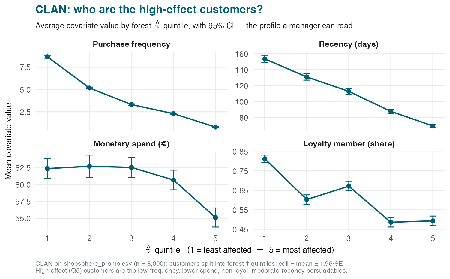
High-effect = low-frequency, recent, non-loyal persuadables; low-effect = loyal regulars. A describable persona — and a sanity check: if the extremes made no business sense, distrust the model.

CLAN gets one slide as the interpretability layer. Once the CATE is validated, take the most- and least-affected groups (top and bottom quantiles of tau-hat) and compare their average covariates. On ShopSphere the high-effect group is the low-frequency, recently-active-but-infrequent (recency below the ~132-day policy cutoff), low-engagement customers — the classic persuadables — while the low-effect group is the loyal regulars who would buy anyway. Two payoffs: it converts an opaque function into a persona a manager can act on and reason about, and it is a sanity check — if the high- and low-effect groups differed on nothing interpretable, or in a direction that contradicts domain knowledge, you should distrust the model regardless of a significant BLP. CLAN is the bridge from a validated estimate to a communicable story.

The validation checklist

Before you act on \(\hat\tau(x)\), clear three gates

1. Real? — BLP differential-prediction \(\beta_2\) significantly \(> 0\). (ShopSphere: 1.08, \(p<2e\text{-}16\) ✓)
2. Worth it? — RATE / AUTOC significantly \(> 0\). (ShopSphere: 5.24, \(t=34\) ✓)
3. Sensible? — CLAN extremes match domain intuition. (persuadables = lapsing customers ✓)

Only an estimate that clears all three earns a policy. A wiggly histogram alone earns nothing.

Consolidate Act 4 into a deployable discipline. Three gates, in order. Real: the BLP differential-prediction coefficient must be significantly positive — the estimate tracks the truth. Worth it: the RATE must be significantly positive — the ranking creates value over a blanket policy. Sensible: the CLAN characterization must agree with domain knowledge — the extremes are who you’d expect. ShopSphere passes all three. The cultural message to leave with students: a flexible model will always hand you a heterogeneous-looking estimate, and producing one is no achievement; the achievement is clearing these three gates. An estimate that fails any gate is not a finding, it is a wiggle. Only a validated estimate is allowed to drive the policy we build next.

From Estimate to Decision: Policy Learning

The deliverable is a rule, not a curve

A manager cannot deploy a histogram. The deliverable is a policy — a function that says, for each customer, treat or not:

\[\pi : X \;\longrightarrow\; \{0, 1\}\]

We judge a policy by its value — the expected outcome if we deploy it:

\[V(\pi) \;=\; \mathbb{E}\big[\,Y(\pi(X))\,\big]\]

The goal of policy learning: find the \(\pi\) that maximizes value subject to constraints (budget, fairness, explainability) — not the \(\pi\) that best estimates \(\tau(x)\).

Pivot from estimation to decision. The output of Acts 3-4 is an estimated, validated CATE — but no one deploys a function or a histogram; they deploy a rule that maps each customer to treat-or-not. That rule is the policy pi(X). The right yardstick is the policy VALUE: the expected outcome if the whole population is treated according to pi. Policy learning seeks the value-maximizing pi, possibly under real-world constraints — a treatment budget (treat only 30%), fairness (don’t condition on protected attributes), explainability (the rule must be auditable). The crucial reframing for the next slide: maximizing value is NOT the same objective as estimating tau(x) accurately, which is why a good CATE estimate does not automatically give a good policy.

Why “treat everyone with \(\hat\tau>0\)” can fail

The naive policy: treat customer \(i\) iff \(\hat\tau(X_i) > 0\). Intuitive — but flawed.

CATE accuracy ≠ policy quality

A learner can have low CATE-MSE yet make bad decisions — what matters for a policy is getting the sign right near the threshold \(\tau(x)=0\), not the magnitude everywhere. (Qian and Murphy 2011)

• Errors far from zero are costly for MSE but irrelevant for the decision.
• Errors near zero are cheap for MSE but flip the decision — exactly where it hurts.

So we should optimize the decision boundary directly, not plug a noisy point estimate into a threshold.

This is the conceptual heart of Act 5 — the distinction between estimation loss and decision loss. The naive plug-in rule (treat where tau-hat > 0) treats the CATE estimate as if it were truth. But CATE-MSE and policy value reward different things. For policy value, all that matters is whether the SIGN is right near the threshold tau=0; a large magnitude error where tau is clearly positive costs MSE but never changes the decision, while a tiny error where tau is near zero is cheap for MSE but flips treat to don’t-treat. So an estimator optimized for MSE may waste its accuracy budget far from the boundary and be sloppy exactly where decisions are made. Qian and Murphy’s insight: optimize the decision boundary directly via weighted classification, rather than thresholding a point estimate. That is the next slide.

Policy value: collect the effect on whom you treat

Since \(\pi\in\{0,1\}\), the deployed outcome is \(Y(\pi(X))=\pi(X)\,Y(1)+(1-\pi(X))\,Y(0)\). Take the expectation — the treat-none baseline drops:

\[V(\pi)=\mathbb E\big[Y(\pi(X))\big]=\underbrace{\mathbb E[Y(0)]}_{\text{treat-none baseline (constant)}}+\;\mathbb E\big[\pi(X)\,\tau(X)\big]\]

Only the second term depends on \(\pi\), so the value-maximizing rule collects the effect \(\tau\) where it treats:

\[\hat\pi=\arg\max_{\pi}\ \mathbb E\big[\pi(X)\,\tau(X)\big]\]

Treat where \(\tau>0\). Two refinements follow — both still in \(\tau\): recenter on a coin flip (the symmetric \(2\pi-1\) form), then — only once the formula is derived — replace the unseen \(\tau\) by the score \(\psi\).

Where the objective comes from, part 1 — deliberately all in population terms, no score yet. Policy value V(pi)=E[Y(pi(X))]. Because pi is 0/1, the deployed outcome is piY(1)+(1-pi)Y(0), so V(pi)=E[Y(0)]+E[pi*tau]. The treat-none baseline E[Y(0)] is identical for every policy, so it drops: the value-maximizing rule maximizes E[pi(X)tau(X)] — collect the treatment effect on whomever you treat, i.e. treat where tau is positive. Keep this in tau on purpose: we have NOT introduced the score yet. Two refinements come next: the next slide recenters this on a coin flip (giving the symmetric 2pi-1 form), and only AFTER that derivation is complete do we introduce the doubly-robust score psi (E[psi|X]=tau) to make it estimable — introducing the score once, at the end, keeps the derivation clean. This is the spine’s fourth appearance: average=ATE, group=GATE, regress=tau(x), weight-a-classifier=policy.

…measured as your edge over a coin flip

Subtract the coin-flip value \(V(\tfrac12)=\tfrac12\mathbb E[Y(1)]+\tfrac12\mathbb E[Y(0)]\) (treating at random — the best rule ignoring \(X\)) — a constant in \(\pi\), so \(\arg\max\) is unchanged:

\[\begin{aligned} \hat\pi=\arg\max_\pi V(\pi) &=\arg\max_\pi\ \mathbb E[Y(\pi)] =\arg\max_\pi\ \mathbb E[Y(\pi)]-\tfrac12\mathbb E[Y(1)]-\tfrac12\mathbb E[Y(0)]\\[2pt] &=\arg\max_\pi\ \mathbb E\big[\pi Y(1)+(1-\pi)Y(0)\big]-\tfrac12\mathbb E[Y(1)]-\tfrac12\mathbb E[Y(0)]\\[2pt] &=\arg\max_\pi\ \mathbb E\big[(\pi-\tfrac12)Y(1)\big]+\mathbb E\big[(\tfrac12-\pi)Y(0)\big] =\arg\max_\pi\ \mathbb E\big[(\pi-\tfrac12)(Y(1)-Y(0))\big]\\[2pt] &=\arg\max_\pi\ 2\,\mathbb E\big[(\pi-\tfrac12)(Y(1)-Y(0))\big] =\arg\max_\pi\ \mathbb E\big[(2\pi-1)(Y(1)-Y(0))\big]\\[2pt] &\overset{\text{LIE}}{=}\ \arg\max_\pi\ \mathbb E\big[(2\pi-1)\,\tau(X)\big] \end{aligned}\]

Sample version, with the score (\(\mathbb E[\psi\mid X]=\tau\)):

\[\boxed{\,\hat\pi=\arg\max_{\pi}\ \tfrac1n\sum_i\big(2\pi(X_i)-1\big)\psi_i\,}\]

The detailed derivation of the (2pi-1) “edge over a coin flip” form. Start from max value, E[Y(pi)] with Y(pi)=piY(1)+(1-pi)Y(0). Subtract the COIN-FLIP VALUE V(1/2)=0.5E[Y(1)]+0.5E[Y(0)] — the value of treating everyone at random with prob 1/2, the best you can do ignoring X. It is constant in pi, so the argmax is unchanged. Expand Y(pi) and group the Y(1) and Y(0) terms: piY(1)-0.5Y(1)=(pi-0.5)Y(1), and (1-pi)Y(0)-0.5Y(0)=(0.5-pi)Y(0). Factor out: (pi-0.5)Y(1)+(0.5-pi)Y(0)=(pi-0.5)(Y(1)-Y(0)). Multiply by 2 (a positive constant, argmax unchanged): 2(pi-0.5)=(2pi-1), so E[(2pi-1)(Y(1)-Y(0))]. Finally, by the law of iterated expectations (LIE), condition on X: E[Y(1)-Y(0) | X]=tau(X), giving E[(2pi-1)tau(X)]; replacing tau by the doubly-robust score psi (E[psi|X]=tau) yields the empirical objective (1/n) sum_i (2pi-1)psi_i.

Two things to stress. (1) The subtracted constant is the coin-flip VALUE 0.5E[Y(1)]+0.5E[Y(0)] (BOTH terms) — that is exactly what makes the (pi-0.5) factoring work; subtracting half the ATE would not. (2) (2pi-1) is the policy’s WAGER: +1 treat, -1 withhold; a coin flip bets +1 and -1 equally and nets zero, so the objective is literally how much you beat a coin flip by betting in the direction of the score. Next slide: the same sum, read as a weighted classification on the sign.

…which is weighted classification on the sign

Split each score into sign × size, \(\psi_i=\operatorname{sign}(\psi_i)\,|\psi_i|\), and three roles appear:

\[\tfrac1n\sum_i\big(2\pi(X_i)-1\big)\psi_i=\tfrac1n\sum_i\underbrace{|\psi_i|}_{\text{weight}}\;\underbrace{\operatorname{sign}(\psi_i)}_{\text{label }y_i}\;\underbrace{\big(2\pi(X_i)-1\big)}_{\text{prediction }\hat y_i}\]

Both \(y_i\) and \(\hat y_i\) live in \(\{-1,+1\}\), so their product is the classification margin: \(\,y_i\hat y_i=+1\) if the policy agrees with the sign (a right call), \(-1\) if it disagrees (a mistake). Maximizing weighted agreement is minimizing weighted misclassification:

\[\hat\pi=\arg\min_{\pi}\ \tfrac1n\sum_i|\psi_i|\,\cdot\,\mathbf 1\big\{\,2\pi(X_i)-1\neq\operatorname{sign}(\psi_i)\,\big\}\]

label \(=\operatorname{sign}(\psi_i)\) (treat the helped, withhold the hurt) · weight \(=|\psi_i|\) (the stakes) · classifier \(=\pi\). The sign/size split makes the weights \(\ge 0\), so any weighted classifier fits it — tree, logistic, SVM. (Athey and Wager 2021)

Answer “why is it a weighted classification.” Take the objective and write each score as its sign times its magnitude, psi = sign(psi)*|psi|. Now read three roles: |psi_i| is a NON-NEGATIVE weight; sign(psi_i) is the LABEL y_i (the correct action — +1 treat if the coupon helps, -1 withhold if it hurts); (2pi-1) is the classifier’s PREDICTION yhat_i. Both label and prediction are +/-1, so their product is the classification MARGIN: +1 when the policy agrees with the sign (a correct decision), -1 when it disagrees (a mistake), weighted by |psi_i|. Maximizing the weighted sum of agreements is identical to minimizing the weighted 0-1 (misclassification) loss — a cost-sensitive binary classification problem. The reason the sign/size split matters and is not just cosmetic: it converts a SIGNED reward into a label plus a NON-NEGATIVE weight, which is exactly what an off-the-shelf weighted classifier needs. So a tree, a weighted logistic regression, or an SVM all solve it — which is why the lab fits a depth-2 rule with rpart / a weighted DecisionTreeClassifier, and policytree is just an EXACT optimizer of this same objective over shallow trees. (Refs: Athey-Wager 2021; the weighted-classification view goes back to Zhao et al.’s outcome-weighted learning and Beygelzimer-Langford cost-sensitive classification.)

The policy tree: a rule you can defend

Restrict \(\pi\) to a shallow decision tree and the value-maximizing rule becomes human-readable: (Zhou, Athey, and Wager 2023)

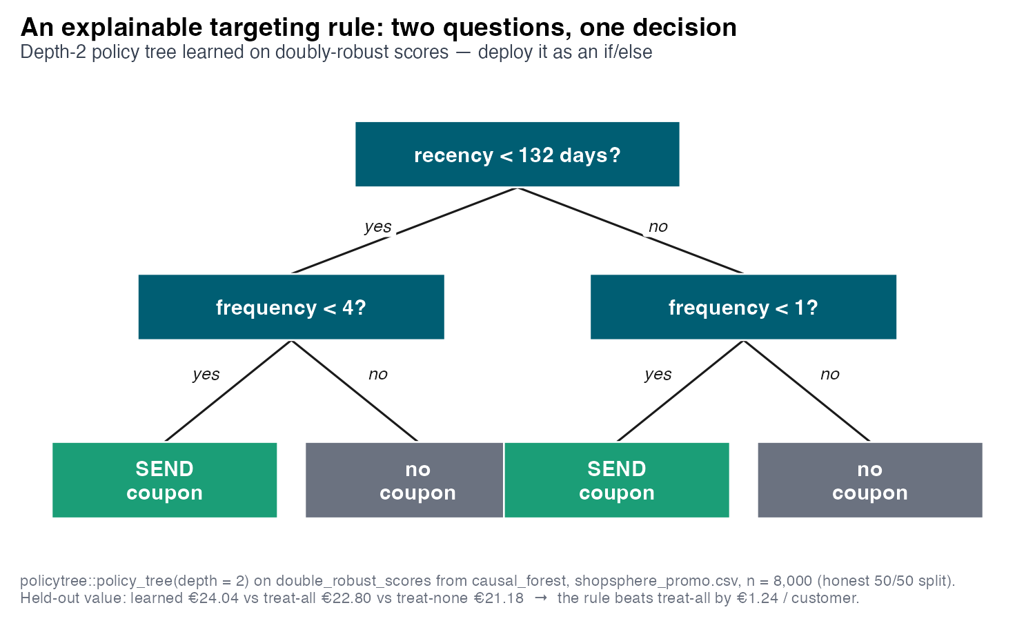
The rule sends the coupon to recent, infrequent buyers (recency < 132 and frequency < 4) and to the lapsed near-one-timer (recency ≥ 132 and frequency < 1) — net-positive since near-zero frequency leaves no margin to cannibalize. Everyone else: withhold — exactly the GATE story.

The policy tree makes the rule auditable (Zhou-Athey-Wager’s policytree optimizes the weighted-classification objective over shallow trees). Constraining the policy class to a depth-2 tree sacrifices a little value for enormous interpretability: the entire targeting rule is two questions. The learned rule on ShopSphere has TWO send-leaves: the dominant one is recency < 132 days AND frequency < 4 purchases (recent but infrequent — reachable yet still persuadable); the second is the lapsed near-one-timer (recency >= 132 AND frequency < 1) — still net-positive on average, because a near-zero purchase frequency leaves no margin to cannibalize, so the coupon can only help (the truly deep-lapsed tail inside this leaf, recency around 270+, is the effect-near-zero “lost-cause” segment). The other two leaves withhold. The common thread is low frequency — leave the loyal regulars alone. Note how it recovers the GATE story (effect falls with frequency) and the CLAN persona (persuadables are low-frequency) as an explicit, deployable rule. A marketing director can read this tree, challenge it, and sign off — which a 0.97-correlation forest, however accurate, does not allow.

The learned policy beats treating everyone

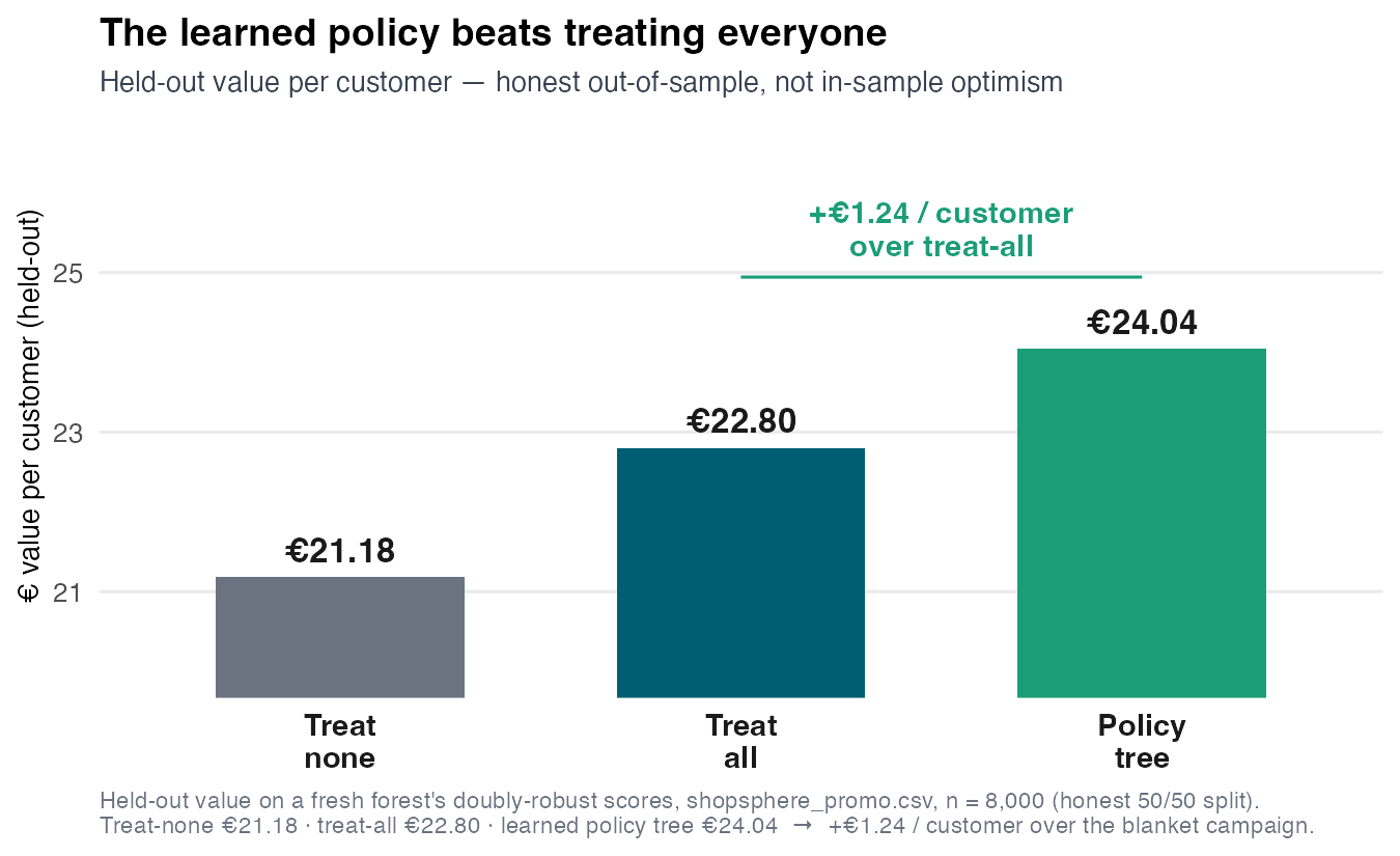
Held-out value per customer: treat-none €21.18 · treat-all €22.80 · policy tree €24.04. The two-question rule beats a blanket campaign by +€1.24 / customer — and beats treating no one by far more.

The value comparison closes the loop and quantifies the payoff, evaluated on held-out data (so it is honest out-of-sample value, not in-sample optimism). Three policies: treat no one yields 21.18 euros per customer (the no-campaign baseline), treat everyone yields 22.80 (the blanket campaign — barely above doing nothing, consistent with the meh 1.5-euro ATE), and the learned depth-2 policy tree yields 24.04. The learned rule beats the blanket campaign by 1.24 euros PER CUSTOMER — across a large customer base that is a substantial sum, generated entirely by withholding the coupon from customers it would hurt. (Python’s DR policy tree shows the same direction, +0.20 on the effect scale; different estimator, same lesson.) This is the entire session monetized: the average said “meh,” heterogeneity said “target,” and targeting turned a near-wash into real profit.

Don’t ship a policy you can’t audit

Before deployment

Report the policy’s value with a confidence interval (is +€1.24 distinguishable from treat-all?), and run CLAN on the policy — who does it treat, who does it withhold from? Audit for fairness and sensibility.

• A policy is a decision that affects people — explainability and a defensible value estimate are not optional.
• Prefer the policy tree (auditable) over a black-box threshold when stakes or scrutiny are high.

The deployment standard: a rule a stakeholder can read, a value they can trust, and a population you can characterize.

End the policy act on governance, not just performance. Two pre-deployment requirements. First, the value gain needs a confidence interval: +1.24 euros is only actionable if it is statistically and practically distinguishable from treat-all — report the uncertainty, do not ship a point estimate. Second, run CLAN on the POLICY itself: characterize who gets treated and who is withheld from, and audit that breakdown for fairness (are we systematically excluding a protected group?) and business sense. The broader principle: a policy is a decision that affects real customers, so auditability and a defensible value estimate are obligations, not niceties — which is the strongest argument for the interpretable policy tree over an opaque threshold whenever scrutiny is high. The deployment bar: readable rule, trustworthy value, characterizable population.

One Score, Four Jobs

Recap: stop averaging, start projecting

• The average lies. A “meh” €1.5 ATE hid effects from −€6.5 to +€20.8 — sign-flipping across customers.
• One score, four jobs. The S08 AIPW \(\psi_i\) (with \(\mathbb{E}[\psi\mid X]=\tau(x)\)): average → ATE (the S08 job); then four new jobs — group → GATE · regress on \(X\) → \(\tau(x)\) · rank → RATE · weight → policy.
• Estimate with orthogonality. Causal forests / DR-learner target \(\tau\) directly — predicting \(Y\) well is not estimating \(\tau\) well.
• Validate before believing. A flexible learner always draws a wiggle: clear BLP (real?), RATE (worth it?), CLAN (sensible?).
• Ship a rule, not a curve. Policy = weighted classification on \(\psi\); the policy tree beat treat-all by +€1.24 / customer.

The five takeaways, each a load-bearing idea. One: the average is the wrong summary when effects are heterogeneous — ShopSphere’s 1.5-euro ATE hid a distribution spanning -6.5 to +20.8 with a sign change. Two: the unifying spine — one AIPW score; averaging it is the S08 ATE, and the four NEW jobs (group/regress/rank/weight) give GATE/tau(x)/RATE/policy; if students remember one thing, this is it. Three: estimate by targeting tau directly with orthogonal methods, because outcome prediction and effect estimation are different objectives. Four: always validate — BLP for realness, RATE for value, CLAN for sense — because flexible learners manufacture heterogeneity. Five: the deliverable is an auditable decision rule, and on ShopSphere it turned a near-break-even campaign into real money. That is the arc: average lies, project the score, validate, decide.

Where this goes next

Closing Part IV — Causal Machine Learning

S08 + S09 are one method: orthogonalize and cross-fit the score, then either average it (ATE) or project it (heterogeneity, targeting, policy).

• Assignment IV (spans S08 + S09): de-confound an observational treatment, estimate and validate its heterogeneity, and recommend a targeting policy.
• Part V — Panel methods. The same orthogonal-score machinery powers Difference-in-Differences with flexible controls — Chang’s DML-DiD. (Chang 2020)

The through-line of the whole course: identify the effect, estimate it honestly, then act on it.

Land the bridge. First, unify the part: S08 and S09 are a single method seen twice — build the orthogonal, cross-fitted score, then choose your operation, average for the ATE or project for everything heterogeneous. Second, point at Assignment IV, which spans both sessions: students de-confound an observational treatment (S08), estimate and VALIDATE its heterogeneity, and recommend a policy (S09) — the validation step is graded heavily because it is what separates a finding from a wiggle. Third, the forward link: Part V moves to panel data, and the same orthogonal-score logic reappears in Chang’s double/debiased DiD, so this machinery is not left behind. Close on the course’s spine: identify, estimate honestly, act.

References

Athey, Susan, and Guido Imbens. 2016. “Recursive Partitioning for Heterogeneous Causal Effects.” Proceedings of the National Academy of Sciences 113 (27): 7353–60. https://doi.org/10.1073/pnas.1510489113.

Athey, Susan, Julie Tibshirani, and Stefan Wager. 2019. “Generalized Random Forests.” The Annals of Statistics 47 (2): 1148–78. https://doi.org/10.1214/18-AOS1709.

Athey, Susan, and Stefan Wager. 2021. “Policy Learning with Observational Data.” Econometrica 89 (1): 133–61. https://doi.org/10.3982/ECTA15732.

Chang, Neng-Chieh. 2020. “Double/Debiased Machine Learning for Difference-in-Differences Models.” The Econometrics Journal 23 (2): 177–91. https://doi.org/10.1093/ectj/utaa001.

Chernozhukov, Victor, Mert Demirer, Esther Duflo, and Iván Fernández-Val. 2018. “Fisher-Schultz Lecture: Generic Machine Learning Inference on Heterogenous Treatment Effects in Randomized Experiments, with an Application to Immunization in India.” https://arxiv.org/abs/1712.04802.

Curth, Alicia, and Mihaela van der Schaar. 2023. “In Search of Insights, Not Magic Bullets: Towards Demystification of the Model Selection Dilemma in Heterogeneous Treatment Effect Estimation.” In Proceedings of the 40th International Conference on Machine Learning (ICML), 202:6623–42. Proceedings of Machine Learning Research.

Kennedy, Edward H. 2023. “Towards Optimal Doubly Robust Estimation of Heterogeneous Causal Effects.” Electronic Journal of Statistics 17 (2): 3008–49. https://doi.org/10.1214/23-EJS2157.

Künzel, Sören R., Jasjeet S. Sekhon, Peter J. Bickel, and Bin Yu. 2019. “Metalearners for Estimating Heterogeneous Treatment Effects Using Machine Learning.” Proceedings of the National Academy of Sciences 116 (10): 4156–65. https://doi.org/10.1073/pnas.1804597116.

Lechner, Michael. 2018. “Modified Causal Forests for Estimating Heterogeneous Causal Effects.” https://arxiv.org/abs/1812.09487.

Nie, Xinkun, and Stefan Wager. 2021. “Quasi-Oracle Estimation of Heterogeneous Treatment Effects.” Biometrika 108 (2): 299–319. https://doi.org/10.1093/biomet/asaa076.

Qian, Min, and Susan A. Murphy. 2011. “Performance Guarantees for Individualized Treatment Rules.” The Annals of Statistics 39 (2): 1180–210. https://doi.org/10.1214/10-AOS864.

Semenova, Vira, and Victor Chernozhukov. 2021. “Debiased Machine Learning of Conditional Average Treatment Effects and Other Causal Functions.” The Econometrics Journal 24 (2): 264–89. https://doi.org/10.1093/ectj/utaa027.

Wager, Stefan, and Susan Athey. 2018. “Estimation and Inference of Heterogeneous Treatment Effects Using Random Forests.” Journal of the American Statistical Association 113 (523): 1228–42. https://doi.org/10.1080/01621459.2017.1319839.

Yadlowsky, Steve, Scott Fleming, Nigam Shah, Emma Brunskill, and Stefan Wager. 2025. “Evaluating Treatment Prioritization Rules via Rank-Weighted Average Treatment Effects.” Journal of the American Statistical Association 120 (549): 38–51. https://doi.org/10.1080/01621459.2024.2393466.

Zhou, Zhengyuan, Susan Athey, and Stefan Wager. 2023. “Offline Multi-Action Policy Learning: Generalization and Optimization.” Operations Research 71 (1): 148–83. https://doi.org/10.1287/opre.2022.2271.

Thank you for your attention!
	www.startupengineer.io/team/ihl/ christoph-ihl christophihl