8. Double Machine Learning

Causal Data Science for Business Analytics

Christoph Ihl

Hamburg University of Technology

Monday, 15. June 2026

S07 went hunting for exogenous variation.

Today we have the opposite luxury: lots of covariates X, and a machine that predicts Y and D beautifully.

Can a black-box predictor hand us a causal effect — with honest error bars?

The cold open frames the whole session. S06 adjusted for measured X by hand; S07 engineered identification with instruments and cutoffs. Today we return to selection-on-observables — we believe X is enough — but X is high-dimensional and the relationships are nonlinear, so we want to let machine learning model the nuisances. The danger: a great predictor is not a great estimator. The session is about the bookkeeping (orthogonality + cross-fitting) that turns ML predictions into a valid causal estimate with a trustworthy confidence interval.

Where DML sits in the toolkit you already have

Same average-effect question as S06 — but the controls go nonparametric. Heterogeneity \(\tau(x)\) is next week.

Orient students before the motivation. DML does not change the causal question relative to S06 — it is still selection-on-observables, still an average effect. What changes is that the control function can be arbitrarily flexible: no more guessing the functional form of g(X). The map’s vertical axis is the S08/S09 boundary: this week we aggregate to an average; next week we let the effect vary with x. Knaus’s maxim belongs here: DML solves the ESTIMATION problem (nuisances), not the IDENTIFICATION problem (you still need unconfoundedness). With the map in hand, the next act motivates why a naive ML plug-in fails.

A Machine That Predicts Is Not a Machine That Explains

What we actually want: a number AND a trustworthy interval

The deliverable is not a point estimate — it is a point with calibrated uncertainty:

\[\sqrt{n}\,(\hat\tau - \tau) \;\xrightarrow{d}\; \mathcal{N}(0, V)\]

That one line demands three things at once:

• consistency — \(\hat\tau \to \tau\),
• \(\sqrt{n}\)-rate — the error shrinks fast enough to matter,
• asymptotic normality — so \(\hat\tau \pm 1.96\,\widehat{\text{SE}}\) has 95% coverage.

A model that only predicts well delivers none of these for \(\tau\) — that is today’s problem.

Hammer the distinction between prediction and estimation. A random forest can predict exam scores with low test error and still give a badly biased, wrongly-scaled estimate of the treatment effect. The target is the sampling distribution of tau-hat: centered on truth, root-n, normal. That is what lets us report a confidence interval we can defend. Everything in the session is in service of recovering that one line while using flexible ML for E[Y|X] and E[D|X].

What we have: a great predictor that converges too slowly

Plug a flexible learner \(\hat g(X)\) into a naive estimator and two biases leak into \(\hat\tau\):

Regularization bias

To control variance, ML shrinks (lasso penalty, shallow trees). That shrinkage is correlated with \(D\) through \(X\) — so it leaks straight into \(\hat\tau\).

Overfitting bias

Evaluate the nuisance on the same rows used to fit it and the model has partly memorised its own noise — biasing \(\hat\tau\) and shrinking its SE.

ML nuisances converge at a slow \(n^{-1/4}\) rate; a naive plug-in inherits that rate for \(\tau\) — far too slow for a \(\sqrt{n}\) CI.

These are the two enemies. Regularization bias: every good ML method trades variance for bias by shrinking, and because the treatment is related to X, that bias doesn’t wash out of the treatment coefficient. Overfitting bias: if the same observations train the nuisance and enter the moment that estimates tau, the in-sample fit is too optimistic. Both vanish under the two ingredients we build today — orthogonality kills the first, cross-fitting kills the second. The n^{-1/4} remark previews why we need orthogonality: it makes tau depend only on the PRODUCT of two slow errors, which is fast enough.

Why a naive ML plug-in is biased — see it once

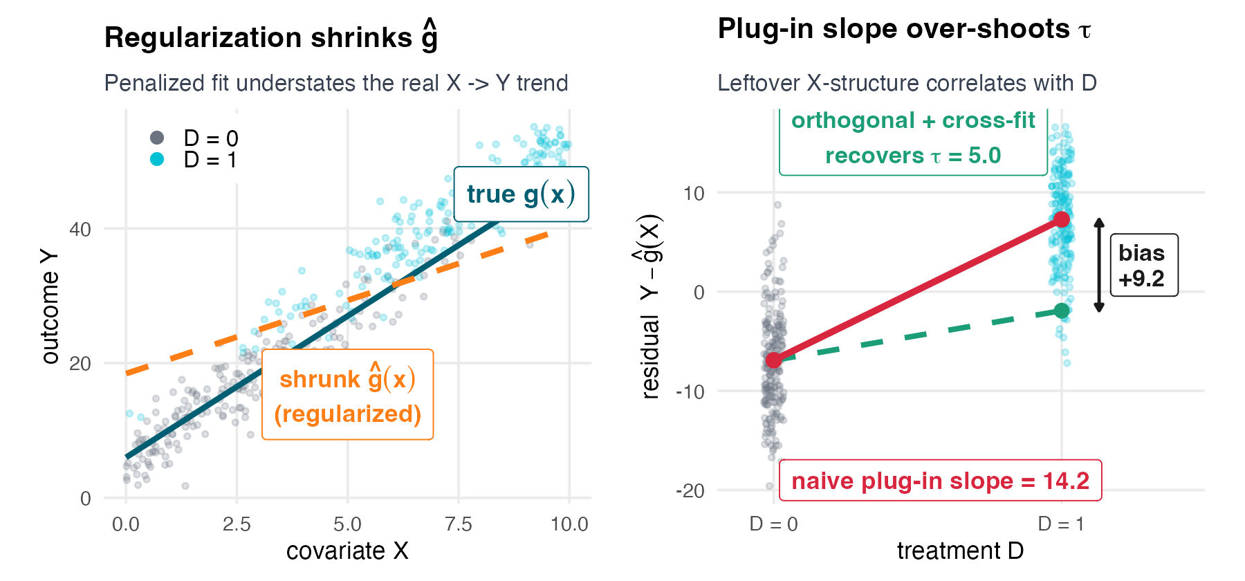
A shrunk \(\hat g(X)\) leaves structure in the residuals that is correlated with \(D\) — and that leftover slope masquerades as a treatment effect. Orthogonalizing + cross-fitting \(Y\) and \(D\) removes it.

This is the picture behind regularization bias. The left panel: a penalized fit is pulled toward the mean, so it systematically under-explains the outcome. The right panel: whatever g-hat failed to remove is still in the residuals, and because D is related to X, that leftover is correlated with D and shows up as a spurious treatment slope. The naive plug-in reads ~14 against a truth of 5. The orthogonal, cross-fitted estimator removes it. Keep “regularization bias” and “overfitting bias” as the two named villains for the rest of the session.

LearnLoop: does the recommender actually lift exam scores?

Symbol	LearnLoop	Role
\(D\)	recommended (0/1)	treatment
\(Y\)	exam_score	outcome
\(X\)	age, region, device, prior courses, baseline score, …	observed covariates

A naive comparison says +14.03 points. But the recommender targets stronger learners — they would have scored higher anyway. The lift is confounded by \(X\), and the confounding runs through a nonlinear interaction (baseline score × prior courses) that a linear control won’t catch.

Ground the abstractions in the running case. LearnLoop is an online-learning platform; the recommender suggests the next module. The learning team wants the causal lift in exam score. The naive treated-minus-control gap is about +14 points, but the targeting rule recommends modules to learners who already had high baselines — classic confounding on observables. Crucially the confounding is nonlinear (an interaction), so we cannot fix it by tossing the covariates into a linear regression. This sets up the punchline three slides from now: linear adjustment gets you to ~5.5 (still off), DML to ~5.0.

The whole session in one recipe

The DML recipe

1. Write a Neyman-orthogonal score for \(\tau\) (insensitive to small nuisance errors).
2. Estimate the nuisances \(g, m\) with any ML learner, using cross-fitting.
3. Solve the empirical moment for \(\hat\tau\).
4. Read the SE off the influence function.

Two ingredients do the real work: orthogonality (kills regularization bias) and cross-fitting (kills overfitting bias). The rest is plumbing.

Give students the map before the territory. Everything today instantiates these four steps. Acts 2–3 build the two ingredients; Act 4 runs the recipe on two models (PLR and AIPW); Act 5 adds a third nuisance for the IV case; Act 6 stress-tests the identifying assumption. Tell them the four-step checklist will reappear verbatim at the end of Act 3.

Partialling-Out: From FWL to Robinson

You already know the trick: Frisch–Waugh–Lovell

To get the coefficient on \(D\) in \(Y \sim D + X\), you do not need the full regression. FWL says: it equals the slope of a residual-on-residual regression.

• Regress \(Y\) on \(X\), keep residuals \(\tilde Y = Y - \hat{E}[Y\mid X]\).
• Regress \(D\) on \(X\), keep residuals \(\tilde D = D - \hat{E}[D\mid X]\).
• Regress \(\tilde Y\) on \(\tilde D\) — that slope is \(\hat\tau\), numerically identical to the full OLS.

“Partial out \(X\), then read the slope.” We met this in S06 (matching) and S07 (2SLS purges \(D\)). Today we swap OLS for ML in the two partialling-out steps. (Frisch and Waugh 1933; Lovell 1963)

FWL is the conceptual hinge and students have seen it. The key reframing: the only role of X in estimating tau is to be partialled out of both Y and D. OLS partials out by linear projection; nothing forces that projection to be linear. If E[Y|X] and E[D|X] are nonlinear, use a learner that captures them. Everything else about FWL is preserved. This is the gentlest possible on-ramp to DML: it is FWL with a better residualizer.

Two kinds of parameter: target vs nuisance

Don’t interpret every coefficient

In \(Y = \tau D + g(X) + \varepsilon\), only \(\tau\) is the target. The function \(g(X)\) is a nuisance — needed for estimation, never interpreted.

This split is liberating: we no longer need a correct, interpretable model of \(g\). We only need to predict it well enough to partial it out.

That is exactly the job ML is good at — and exactly why we can hand \(g\) to a black box without guilt.

This is a mindset shift from a regression course where every coefficient gets a story. In causal ML, g(X) is scaffolding: it exists only so that tau is identified, and we judge it purely by predictive quality, not interpretability or correct specification. This is what licenses the use of opaque learners. It also previews double robustness: because g is a nuisance, we are allowed to be wrong about it in ways that don’t contaminate tau — if we use the right (orthogonal) score.

The partially linear model (Robinson, 1988)

Treatment enters linearly; the controls enter arbitrarily — that’s what partially linear means. (Robinson 1988)

\[Y = \tau\, D + g(X) + \varepsilon, \qquad \mathbb{E}[\varepsilon \mid D, X] = 0\] \[D = m(X) + \nu, \qquad \mathbb{E}[\nu \mid X] = 0\]

• \(\tau\) — the target (constant treatment effect, the ATE).
• \(g(X)\) — the structural outcome function.

We partial out the two nuisances:

• \(\ell(X)=\mathbb{E}[Y\mid X]=\tau\,m+g\) — the reduced-form outcome (not \(g\)).
• \(m(X)=\mathbb{E}[D\mid X]\) — the propensity.

Write the model cleanly. The partially linear model keeps the treatment linear (one number tau) but lets g and m be anything. Then name the two things we actually estimate and remove — the nuisances: l(X) = E[Y|X], the reduced-form outcome predictor (NOT the structural g; l = tau*m + g folds in the indirect path X drives D drives Y), and m(X) = E[D|X], the propensity. We stop here at WHAT gets partialled out; the actual subtraction that cancels g and leaves a residual-on-residual relation is the very next slide. That residualized relation is Robinson’s partialling-out estimator, the PLR score DoubleML uses (ml_l and ml_m).

Partialling-out, annotated

\[\hat\tau \;=\; \frac{\widehat{\text{Cov}}(\tilde Y,\ \tilde D)}{\widehat{\text{Var}}(\tilde D)}, \qquad \tilde Y = Y - \hat\ell(X),\quad \tilde D = D - \hat m(X)\]

• \(\tilde Y\) — the part of the exam score not predicted by who the learner is.
• \(\tilde D\) — the part of the recommendation not predicted by who the learner is (the as-good-as-random slice).
• The slope of \(\tilde Y\) on \(\tilde D\) is the treatment effect, purged of \(X\).

Here \(\hat\ell(X) = \hat{\mathbb{E}}[Y\mid X]\) is the reduced-form outcome predictor — \(\ell = \tau\,m + g\), folding in the indirect path of \(X\) through \(D\). It is DoubleML’s ml_l (not the structural \(g\)).

Make every symbol concrete in LearnLoop terms. Y-tilde is the exam score with the predictable-from-X part removed; D-tilde is the recommendation with the predictable-from-X part removed — the residual variation in treatment that is not explained by who the learner is. Regressing one residual on the other isolates the effect. Note carefully that the outcome nuisance here is the REDUCED FORM E[Y|X] (often written l(X)), not the structural g(X); DoubleML’s PLR uses ml_l for exactly this. Students who conflate the two get confused later, so name it now.

The leap: swap OLS for any ML learner

OLS partials out \(X\) by a linear projection. Nothing requires that.

Residualize with…	\(\hat{\mathbb{E}}[Y\mid X]\), \(\hat{\mathbb{E}}[D\mid X]\)
Linear regression	only linear/additive structure
Random forest, lasso, boosting, neural net	arbitrary nonlinearity + interactions

In LearnLoop the confounding hides in a baseline-score × prior-courses interaction. A linear control misses it; a random forest catches it — and the residual-on-residual slope snaps onto the truth.

This is the moment DML is born. The two partialling-out regressions are just conditional-expectation estimates, and we can estimate a conditional expectation with anything. The table contrasts the linear residualizer (which can only remove linear confounding) with flexible learners (which remove whatever structure is there). Tie it to LearnLoop: the confounding is an interaction, invisible to linear adjustment, visible to a forest. That is precisely why linear OLS lands at 5.5 and DML at 5.0 — preview the next slide’s figure.

See it on LearnLoop: let the machine remove X, then read the slope

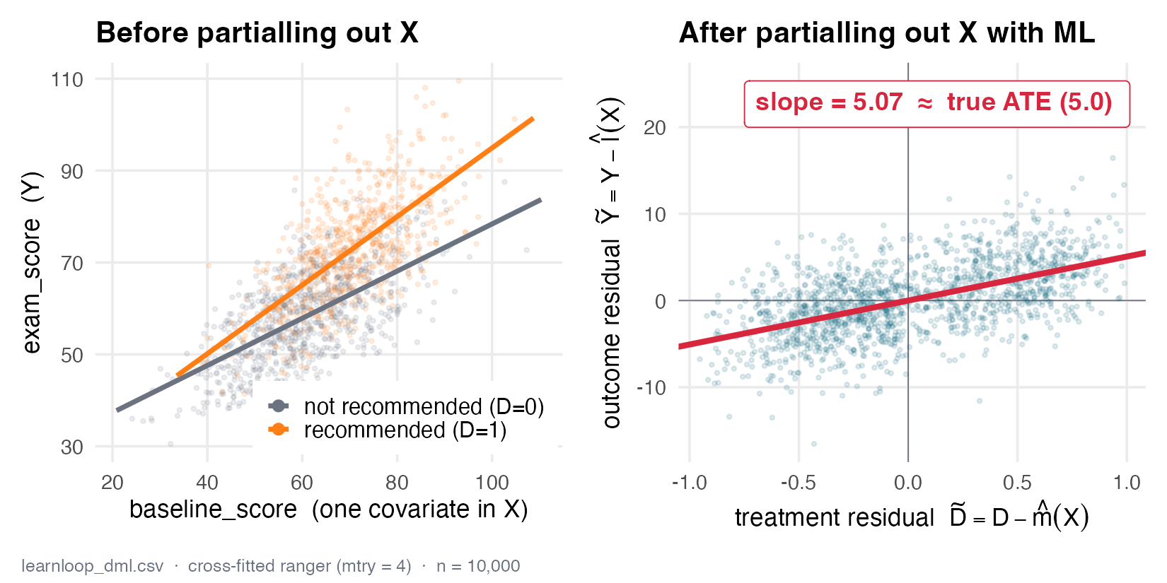
Left: treated learners sit higher partly because of \(X\). Right: after ML residualization, the slope of \(\tilde Y\) on \(\tilde D\) is ≈ 5.0 — the partialling-out estimate.

The picture pays off the algebra. On the left, the raw association is contaminated: treated points are higher because the recommender targets high-baseline learners. On the right, once X is partialled out with a cross-fitted forest, the residual cloud has a clean slope of about 5 — the true effect. This is the PLR estimator in one figure, and it is exactly what DoubleMLPLR computes. Next act: why we needed orthogonality and cross-fitting to make this trustworthy rather than merely suggestive.

Two Ingredients: Orthogonality + Cross-Fitting

What is a score? An estimating equation for \(\tau\)

Score (moment function)

A score \(\psi(W;\tau,\eta)\) ties together the data \(W=(Y,D,X)\), the target \(\tau\), and the nuisances \(\eta=(\ell,m)\). Its moment — the population expectation — is zero at the truth: \(\;\mathbb{E}[\psi(W;\tau_0,\eta_0)]=0\), which pins down \(\tau_0\).

Every score here is linear in \(\tau\): \(\;\psi=\psi_a(W;\eta)\,\tau+\psi_b(W;\eta)\), so the root is closed-form, \(\hat\tau=-\mathbb{E}_n[\psi_b]/\mathbb{E}_n[\psi_a]\) (ML \(\hat\eta\) plugged in).

Partialling-out is an exact example of this:

\[\psi=(\tilde Y-\tau\tilde D)\,\tilde D=\underbrace{(-\tilde D^{2})}_{\psi_a}\,\tau+\underbrace{\tilde Y\tilde D}_{\psi_b}\;\Rightarrow\;\tau=\frac{\mathrm{Cov}(\tilde Y,\tilde D)}{\mathrm{Var}(\tilde D)}\]

The two ingredients: orthogonality (a property of this score) and cross-fitting (how \(\hat\eta\) enters it).

Name the central object before using it. A score (estimating equation / moment function) is a function of the data, the target tau, and the nuisances whose EXPECTATION is zero at the true parameter — that zero-expectation statement is the “moment condition,” and it identifies tau. Key structural fact: every DML score here is LINEAR in tau, psi = psi_atau + psi_b, so we never iterate — the estimator is just tau_hat = -E_n[psi_b]/E_n[psi_a], with ML nuisances and a sample average plugged in. For PLR, psi_a = -Dtilde^2 and psi_b = YtildeDtilde — which are EXACTLY DoubleML’s internal psi_a / psi_b — and the ratio is the Cov/Var slope from the partialling-out slide. So we ALREADY met a score. Saying this out loud lets the next two slides land — orthogonality is a property OF this score (its first-order sensitivity to nuisance error), and cross-fitting is HOW we plug the ML nuisances in. Nuisances are (l, m) = (E[Y|X], E[D|X]), matching ml_l / ml_m, not g.

Step 1 — an orthogonal score (Neyman orthogonality)

Orthogonality

A score is Neyman-orthogonal if slightly-wrong nuisance models barely move the estimate: its sensitivity to nuisance error is zero to first order — the linear (\(\delta\)) term cancels, leaving only a second-order (\(\delta^2\)) effect.

Formally, the moment \(\psi(W;\tau,\eta)\) has zero Gateaux derivative in the nuisance \(\eta=(\ell,m)\) at the truth:

\[\left.\partial_{\eta}\, \mathbb{E}\big[\psi(W;\tau_0,\eta)\big]\right|_{\eta=\eta_0} = 0\]

Consequence: the bias in \(\hat\tau\) depends on the product of the two nuisance errors, not their sum. Two slow \(n^{-1/4}\) errors multiply to \(n^{-1/2}\) — fast enough for a valid CI.

This is the conceptual heart, and both standard references under-explain the intuition, so lead with words. Orthogonality means: if your propensity model or outcome model is slightly off, the treatment estimate barely budges — the score is built so the first-order sensitivity is zero. The payoff is the product structure: instead of bias ~ (error in l) + (error in m), orthogonality gives bias ~ (error in l) × (error in m). Each ML error is O(n^{-1/4}); the product is O(n^{-1/2}), which is exactly the rate a root-n CI needs. The partialling-out (Robinson) score is orthogonal; the naive plug-in is not. Full Gateaux-derivative derivation is in the session notes.

Orthogonality, drawn

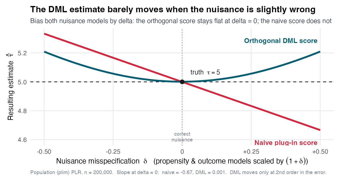
Perturb the nuisances by \(\delta\). The naive score cuts steeply through the truth (slope \(\ne 0\)). The orthogonal score is flat at \(\delta = 0\) — it only feels the error at second order.

This figure is the visual definition of orthogonality. The horizontal axis is how wrong the nuisance models are; the vertical axis is the resulting estimate. The naive plug-in is a straight line through the truth with a real slope: small nuisance error -> proportional estimate error. The orthogonal score sits at the bottom of a parabola: its slope at delta=0 is zero, so small nuisance errors cost you essentially nothing. That flatness is what makes ML nuisances safe to use. Numbers in the caption: naive slope -0.67, DML slope 0.001.

Step 2 — cross-fitting kills the overfitting bias

The danger: if the same rows train the nuisance and enter the moment for \(\tau\), the model has seen its own noise.

The cross-fitting mantra

A unit must never be predicted by a model that was trained on it.

So we split the sample: fit \(\hat g, \hat m\) on other folds, predict the held-out fold, and rotate until every unit has an out-of-fold prediction. Out-of-fold predictions are independent of each unit’s own noise — the overfitting bias vanishes.

The second ingredient is mechanical but essential. Even with an orthogonal score, reusing the training rows to evaluate the moment reintroduces bias through own-observation overfitting — and it also makes the SE too small, so CIs under-cover. Cross-fitting is the fix: predictions for a unit always come from a model that never saw it. This decouples the nuisance estimation error from the moment evaluation. Emphasize it is not optional polish; it is what makes the SE honest.

Cross-fitting, drawn

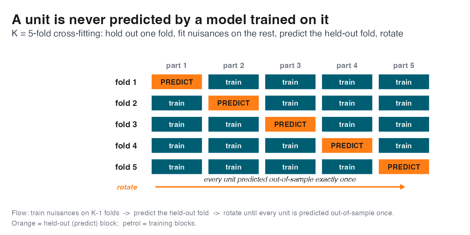
Five folds: each part is predicted by a model trained on the other four — so every unit is predicted out-of-sample exactly once, never by a model that saw it.

Walk the grid one row at a time. Row 1: train on parts 2–5, predict part 1. Row 2: train on parts 1,3,4,5, predict part 2. And so on. After five rotations, every observation has exactly one out-of-fold prediction, and those stack into the residuals that feed the moment. Averaging across folds (and, in practice, across repetitions) stabilizes the estimate. This is the operational meaning of the mantra on the previous slide.

How many folds — and why repeat?

• Five folds is the workhorse default (2 is fine for huge \(n\); more folds = more training data per fold, more compute).
• The fold split is random — a single split adds noise. Repeat the whole cross-fitting \(n_{\text{rep}}\) times and take the median estimate / aggregate the SEs.
• Use a genuinely flexible learner (random forest, boosting); don’t pre-commit to one — stack / super-learn if unsure. (Ahrens et al. 2025)

In LearnLoop the key knob is the forest’s mtry: too small and it can’t see the interaction — the estimate drifts. Tuning matters because the nuisance quality is what orthogonality leans on.

Practical guidance students will need in the lab. Five folds balances bias and compute. Because the split is random, report a repeated-cross-fitting estimate (median over n_rep) so your answer isn’t an artifact of one partition. On learner choice: there is no need to gamble — Ahrens et al. show you can stack several learners inside DML and let the data weight them. The mtry remark is a real lesson from this dataset: with the default mtry the forest misses the baseline-score × prior-courses interaction and the estimate biases upward; bumping mtry fixes it. Orthogonality buys robustness to SMALL nuisance error, not to a learner that fundamentally can’t fit the surface.

The payoff: only orthogonality AND cross-fitting work

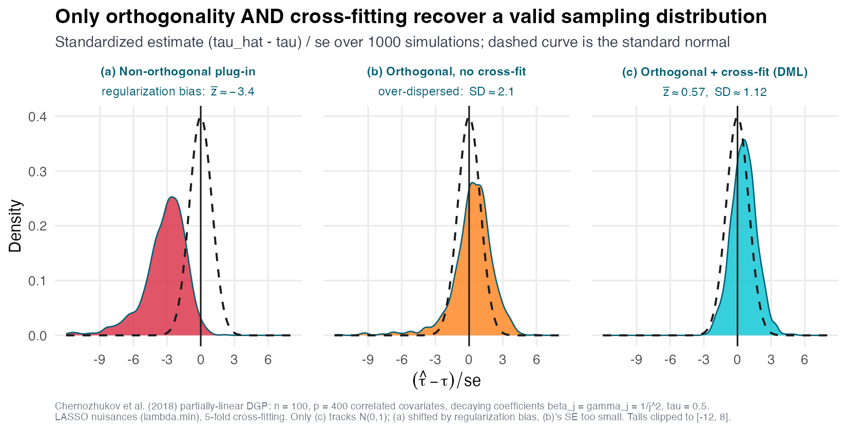
(a) non-orthogonal → shifted (regularization bias). (b) orthogonal, no cross-fit → over-dispersed (SE too small). (c) orthogonal + cross-fit → centered, correctly scaled \(\mathcal{N}(0,1)\).

This is the money slide — the empirical proof that you need BOTH ingredients. Standardized estimates (tau-hat minus tau over SE) should look like a standard normal if inference is valid. Panel (a): drop orthogonality and the distribution is shifted off zero — biased. Panel (b): keep orthogonality but skip cross-fitting and the spread is too wide relative to the normal — the SE is wrong, so CIs under-cover. Panel (c): with both, the histogram hugs N(0,1) — valid point estimate AND valid interval. Neither ingredient alone suffices. This is Chernozhukov et al. (2018) in one figure.

Step 3 — average the per-unit scores into \(\hat\tau\)

Each unit has a per-unit score \(\psi_i=\psi(W_i;\tau,\hat\eta_{-k(i)})\) — its own out-of-fold nuisances — and it is linear in \(\tau\): \(\psi_i=\psi_{a,i}\,\tau+\psi_{b,i}\).

Set the average to zero and solve:

\[\mathbb{E}_n[\psi]=0\quad\Longrightarrow\quad \hat\tau=-\frac{\mathbb{E}_n[\psi_b]}{\mathbb{E}_n[\psi_a]}\qquad\text{(average the pieces, then divide).}\]

Robinson PLR — \(\psi_{a,i}=-\tilde D_i^{2},\ \psi_{b,i}=\tilde Y_i\tilde D_i\):\(\quad\hat\tau=\dfrac{\overline{\tilde Y\tilde D}}{\overline{\tilde D^{2}}}=\dfrac{\mathrm{Cov}(\tilde Y,\tilde D)}{\mathrm{Var}(\tilde D)}\).

Same crank everywhere — only \(\psi\) changes: AIPW (\(\psi_a=-1\)) makes \(\hat\tau=\overline{\psi_b}\) a plain average of scores; IV is a ratio of two averaged scores (Wald).

This is step 3 made explicit. Every unit contributes a per-unit score evaluated at its OWN out-of-fold nuisances. Because the score is linear in tau, the empirical moment — the average of the per-unit scores set to zero — has a closed-form root: tau-hat = -mean(psi_b)/mean(psi_a). For Robinson partialling-out that is mean(Ytilde*Dtilde)/mean(Dtilde^2) = the Cov/Var slope. The generalization is the punchline: AIPW has psi_a = -1, so tau-hat is literally the average of the per-unit scores; IV is a ratio of two averaged scores (Wald). Same averaging machine, different score.

Step 4 — the SE comes from the influence function

A good estimator is asymptotically linear: \(\hat\tau-\tau\approx\frac1n\sum_i\phi(W_i)\). The influence function \(\phi_i\) measures how much unit \(i\) tips the estimate; for DML it is the normalized score:

\[\phi_i=-\frac{\psi_i}{\mathbb{E}[\psi_a]}\ \ (\text{mean }0)\quad\Rightarrow\quad \sqrt{n}\,(\hat\tau-\tau)\xrightarrow{d}\mathcal N\!\big(0,\ \mathbb{E}[\phi^2]\big),\qquad \widehat{\mathrm{SE}}=\sqrt{\tfrac{\mathbb{E}_n[\psi^2]}{\mathbb{E}_n[\psi_a]^{2}\,n}}\]

Robinson: \(\phi_i=\dfrac{(\tilde Y_i-\tau\tilde D_i)\,\tilde D_i}{\mathrm{Var}(\tilde D)}\) — exactly the robust SE of the residual-on-residual regression. Same formula for PLR, AIPW, IV; only \(\psi,\psi_a\) change (AIPW \(\psi_a=-1\Rightarrow\widehat{\mathrm{SE}}=\sqrt{\widehat{\mathrm{Var}}(\psi_i)/n}\)).

This is step 4 — where the standard error comes from. An asymptotically linear estimator can be written as a sample average of an influence function phi_i, so the CLT gives root-n asymptotic normality with variance E[phi^2]. For DML the influence function is the normalized score, phi_i = -psi_i / E[psi_a]; its variance gives SE = sqrt(E_n[psi^2] / E_n[psi_a]^2 / n). For Robinson this is exactly the heteroskedasticity-robust SE of the residual-on-residual regression — reassuringly familiar. It is the SAME formula for PLR, AIPW, IV; only psi and psi_a change. For AIPW (psi_a = -1) it reduces to the ordinary SE of the mean of the per-unit scores. This is why the DML interval is valid: it is the spread of the influence function, not a naive plug-in that ignores nuisance estimation.

The recipe, as a four-step checklist

DML in four steps

1. Orthogonal score — choose a Neyman-orthogonal \(\psi(W;\tau,\eta)\), linear in \(\tau\): \(\;\psi=\psi_a(W;\eta)\,\tau+\psi_b(W;\eta)\).
2. Cross-fitted nuisances — fit \(\hat\eta\) on held-out folds; every unit predicted out-of-fold.
3. Average & solve — \(\mathbb{E}_n[\psi]=0\ \Rightarrow\ \hat\tau=-\,\mathbb{E}_n[\psi_b]\,/\,\mathbb{E}_n[\psi_a]\).
4. Influence-function SE — \(\phi_i=-\,\psi_i/\mathbb{E}_n[\psi_a]\), so \(\;\widehat{\text{SE}}=\sqrt{\mathbb{E}_n[\psi^2]\,/\,\mathbb{E}_n[\psi_a]^2\,/\,n}\).

Memorise this: only the score \(\psi\) (step 1) changes across models (PLR, AIPW, IV) — steps 2–4 are identical. (Chernozhukov et al. 2018)

Throughout the course the effect is \(\tau\); the DML papers and the DoubleML package write it \(\theta\) (reported as coef) — same object.

Consolidate. This checklist is the entire method, and it generalizes: switch the score and you switch the estimand, but steps 2–4 are identical. PLR uses the partialling-out score; AIPW uses the doubly-robust score; IV adds a third nuisance. Tell students that if they remember one slide from today, this is it. The influence-function SE is what makes the interval valid — it is the variance of the score, not a naive plug-in.

AIPW: the Doubly-Robust Score

When the effect isn’t a single number: the interactive model

Same two equations as PLR — but drop the linearity in \(D\):

\[Y=\mu(D,X)+\varepsilon, \qquad \mathbb{E}[\varepsilon\mid D,X]=0\] \[D=e(X)+\nu, \qquad \mathbb{E}[\nu\mid X]=0\]

• \(\mu(D,X)=\mathbb{E}[Y\mid D,X]\) — the outcome surface (arms \(\mu_1(X)=\mu(1,X)\), \(\mu_0(X)=\mu(0,X)\)).
• \(e(X)=\mathbb{E}[D\mid X]\) — the propensity (PLR’s \(m\)).
• No constant \(\tau\): the effect \(\mu_1(X)-\mu_0(X)\) may vary with \(X\).
  • we target the ATE \(=\mathbb{E}[\mu_1(X)-\mu_0(X)]\).

Plug-in alone (\(\overline{\hat\mu_1-\hat\mu_0}\)) inherits the regularization bias → need an orthogonal score: AIPW.

Motivate the second model as PLR with the linearity in D dropped. PLR wrote Y = tau*D + g(X): D enters LINEARLY through one constant tau. The interactive model writes Y = mu(D,X): D enters ARBITRARILY, so the per-unit effect mu1(X) - mu0(X) can vary with X. The propensity equation is unchanged, D = e(X) + nu (e is exactly PLR’s m). This week we target the AVERAGE of those gaps — the ATE = E[mu1 - mu0]; S09 estimates the varying tau(x) itself. The naive plug-in, mean(mu1-hat - mu0-hat), is NOT orthogonal — it carries the regularization bias. The fix is the augmented IPW (AIPW) score: orthogonal and doubly robust. Next slide.

AIPW = Direct estimate + Residual correction

\[\psi_i = \underbrace{\big[\hat\mu_1(X_i) - \hat\mu_0(X_i)\big]}_{\text{direct (outcome regression)}} + \underbrace{\frac{D_i\,(Y_i - \hat\mu_1)}{\hat e(X_i)} - \frac{(1-D_i)(Y_i - \hat\mu_0)}{1-\hat e(X_i)}}_{\text{bias correction (propensity-weighted residual)}}\]

\[\widehat{\text{ATE}} = \frac{1}{n}\sum_i \psi_i\]

The outcome model gives a first guess; the propensity-weighted residual repairs whatever the outcome model got wrong. (Robins, Rotnitzky, and Zhao 1994; Bang and Robins 2005)

Decompose the AIPW score the Athey–Wager way: a direct part (the regression imputation of the gap) plus a correction part (the IPW-weighted residual). The correction term is the genius: wherever the outcome model mis-predicts, the weighted residual pushes back. When the outcome model is right, the residuals are zero in expectation and the correction adds only noise; when it’s wrong, the correction carries the estimate. This is the structural reason for double robustness on the next slide, and it is also exactly the score whose per-unit value we’ll hand to S09.

AIPW slots into the same four steps

The per-unit AIPW signal \(\psi_i\) (last slide) is the score’s \(\psi_b\); subtract \(\tau\) for the orthogonal score:

\[\psi=\psi_i-\tau\qquad\Longrightarrow\qquad \psi_b=\psi_i,\quad \psi_a=-1\]

• Step 2 — nuisances \(\eta=(\mu_1,\mu_0,e)\): now three (PLR’s \(m\) → two arms \(+\) propensity), cross-fitted.
• Step 3 — average & solve \(\hat\tau=-\mathbb{E}_n[\psi_b]/\mathbb{E}_n[\psi_a]=\mathbb{E}_n[\psi_i]\): a plain average of the per-unit signals.
• Step 4 — SE \(\widehat{\text{SE}}=\sqrt{\widehat{\text{Var}}(\psi_i)/n}\) (influence function \(=\psi_i-\bar\psi\)).

Only the score changed — orthogonality (\(=\) double robustness, next) and cross-fitting carry over verbatim.

Double robustness: right if EITHER nuisance is right

Two shots on goal

The AIPW estimate is consistent if either the outcome models \(\mu_1,\mu_0\) or the propensity \(e\) is correctly specified — you don’t need both.

Orthogonality is why: the score’s first-order sensitivity to each nuisance is zero, so an error in one is absorbed as long as the other holds. Double robustness is orthogonality, viewed from the modelling side.

Double robustness is the headline property and students should see it is not a separate magic trick — it is the same orthogonality from Act 3 read through a modelling lens. Two independent chances to be right: get the outcome surface right OR get the propensity right. The connection: zero first-order sensitivity to each nuisance means a wrong nuisance enters only through the product with the other’s error, so if one error is zero the bias is zero. This is the most exam-worthy idea of the act.

AIPW’s bias–variance payoff

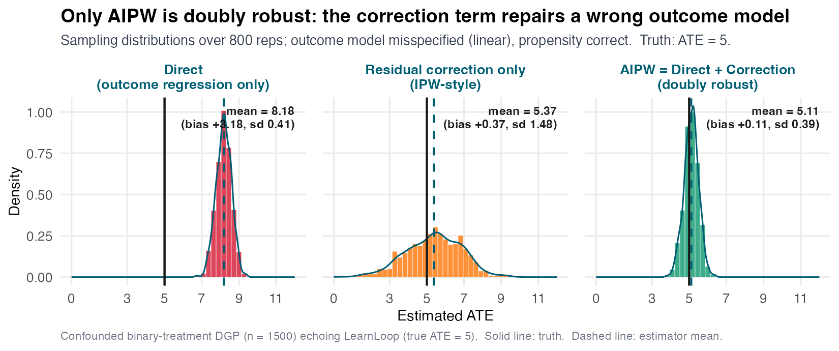
Outcome model misspecified on purpose: Direct is biased (≈ 8.2), IPW-only is centered but noisy, AIPW is centered on 5 and tightest.

The simulation makes double robustness visceral. We deliberately break the outcome model (fit it linear when the truth is nonlinear) but keep the propensity correct. Direct (outcome regression only) is badly biased — it trusts the broken model. IPW-only (the correction term alone) is unbiased but high-variance — it throws away the outcome model’s information. AIPW combines them: the correction repairs the bias, the direct part tames the variance, and you get a tight distribution centered on truth. This is why AIPW is the default for an ATE under unconfoundedness.

Before you trust the weights: check overlap

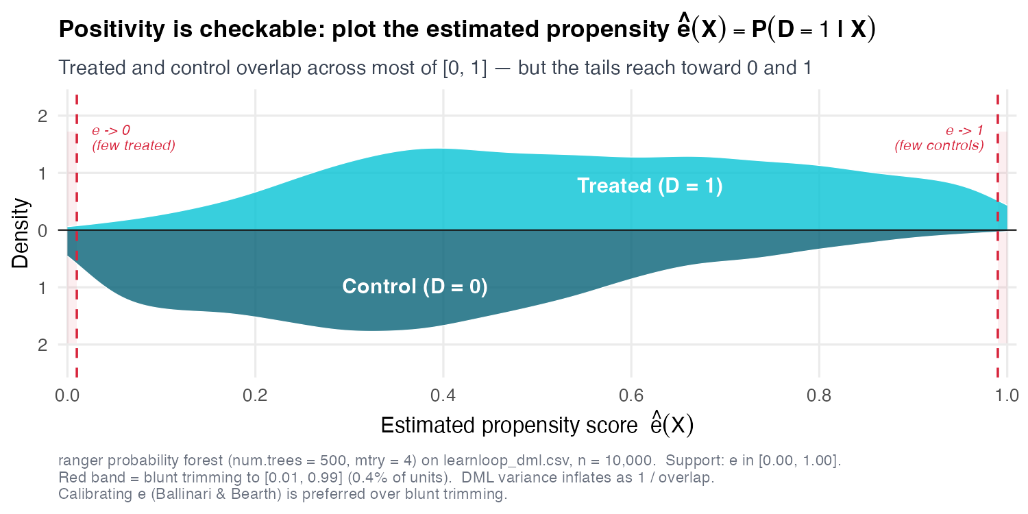
AIPW divides by \(\hat e\) and \(1-\hat e\) — as \(\hat e\to 0,1\) the weights, and the variance, blow up. Always plot this first; then the question is calibrate or trim (next).

Positivity is the assumption that bites AIPW hardest. The correction term has e(X) in the denominator, so units with propensity near 0 or 1 get enormous weights and blow up the variance. The diagnostic is simple and you should always run it: plot the estimated propensity by treatment group and look for overlap. LearnLoop overlaps across most of [0,1] but has tails — realistic. Keep this slide as the pure diagnostic: plot the estimated propensity by group, look for mass piling up near 0 or 1. The next slide formalizes the two cures — calibration (fix the weights) vs trimming (change the estimand).

Trim, clip, or calibrate? Change the question vs. fix the weights

Three responses when AIPW weights \(1/\hat e\) explode as \(\hat e\to 0,1\):

	what it does to \(\hat e\)	estimand	use when
Trim	drops units with \(\hat e\notin[\alpha,1-\alpha]\)	overlap-ATE \(\neq\) ATE	genuine non-overlap
Clip	caps \(\hat e\) at \([\alpha,1-\alpha]\), keeps units	full ATE, capped units biased	quick blunt guard
Calibrate	rescales \(\hat e\to\tilde e\) so \(\mathbb{E}[D\mid\tilde e]=\tilde e\)	full ATE, honest weights	ML over-confidence

Only trim changes the question; clip & calibrate keep the full ATE — clip patches the symptom, calibrate fixes the cause. → Calibrate first. (Ballinari and Bearth 2024; Crump et al. 2009)

Three responses to the weight blow-up, and what each one changes. TRIM changes the estimand: drop units with propensity outside [alpha, 1-alpha] (Crump et al. give an optimal alpha) and you now estimate the ATE only on the overlap subpopulation — a narrower question than the full-population ATE. CLIP (truncation) keeps every unit but caps e-hat at the band, so the capped units carry a deliberately wrong propensity — it patches the symptom (huge weights), and is DoubleML’s default trimming_rule=‘truncate’. CALIBRATE keeps every unit and rescales e-hat to honest values: a model is calibrated if, among units with predicted score p, a fraction p are actually treated, E[D | e-tilde] = e-tilde; flexible ML is over-confident in the tails, so a monotone recalibration (isotonic or Platt; Ballinari–Bearth 2024) pulls scores back, shrinking the inflated 1/e weights without dropping anyone — the full ATE is preserved. Bottom line: only trimming changes the question; clip and calibrate keep the full estimand, but clip is blunt while calibrate fixes the cause. The lab demos all three on LearnLoop.

When Unconfoundedness Fails: DML-IV

If a confounder is unobserved, bring back the instrument

Connect back to last week. DML’s nuisances solve the estimation problem under unconfoundedness; they do nothing about an unobserved confounder. LearnLoop’s lesson-COMPLETION decision is the canonical case: student motivation u drives both completing and exam score, so selection-on-observables fails. The escape is the same as S07 — a valid instrument, here a randomly-timed reminder. The new content this week is only the ML-nuisance layer; identification (relevance, exclusion, monotonicity) is exactly S07’s and we cite it.

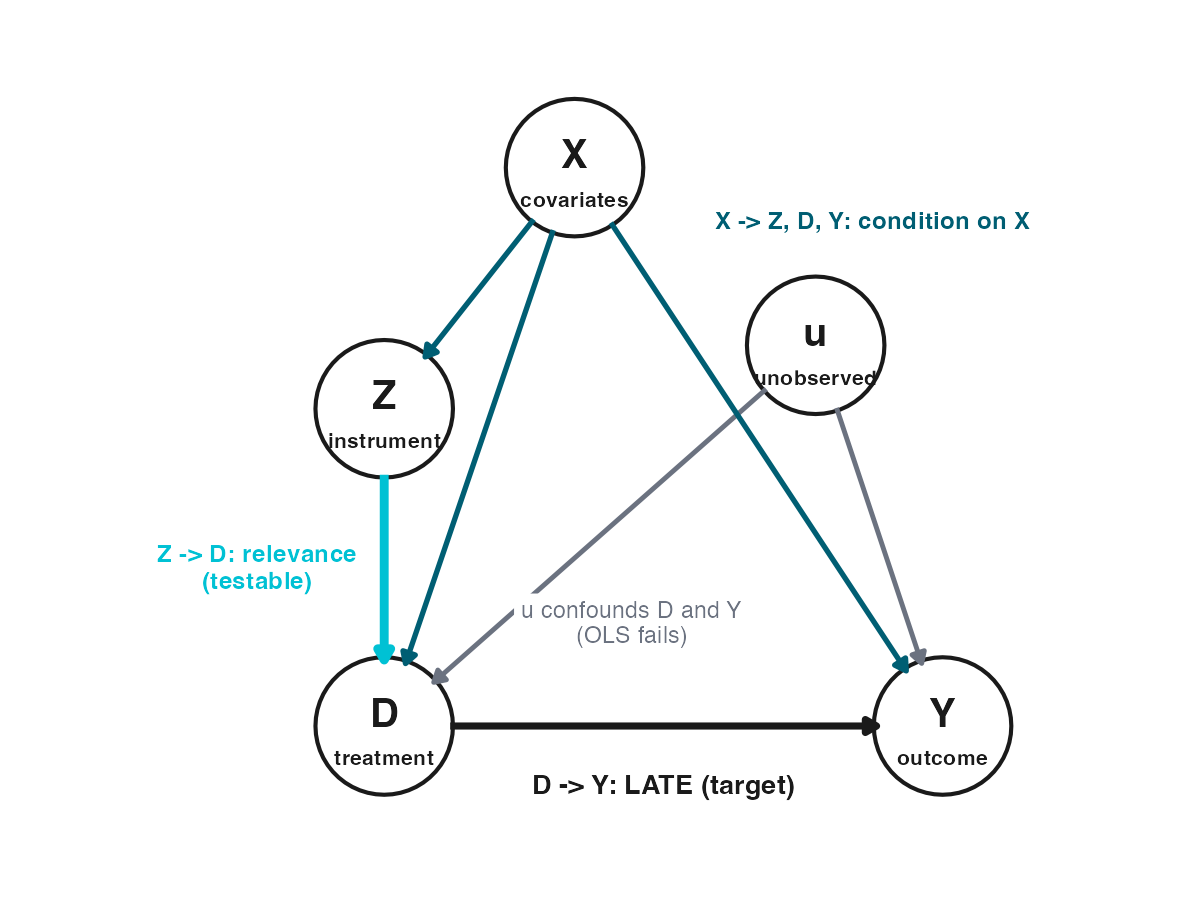
Partially linear IV — the model and the score

\(D\) is endogenous (\(u\) leaks in) — residualize on \(X\) and instrument with \(Z\) (exogeneity on \(Z\), not \(D\)):

\[Y=\tau D+g(X)+\varepsilon,\qquad \mathbb{E}[\varepsilon\mid Z,X]=0\] \[Z=r(X)+\nu,\qquad \mathbb{E}[\nu\mid X]=0\]

• Three nuisances: \(\ell=\mathbb{E}[Y\mid X]\), \(m=\mathbb{E}[D\mid X]\), \(r=\mathbb{E}[Z\mid X]\) — residuals \(\tilde Y,\tilde D,\tilde Z\).
• The orthogonal score uses \(\tilde Z\) as the instrument:

\[\psi=(\tilde Y-\tau\tilde D)\,\tilde Z=\underbrace{(-\tilde D\tilde Z)}_{\psi_a}\,\tau+\underbrace{\tilde Y\tilde Z}_{\psi_b}\]

PLR with one change — \(\psi_a=-\tilde D\tilde Z\) instead of \(-\tilde D^2\): instrument the residual. (Robinson 1988)

Page 1: the model and the score. D is endogenous (the unobserved u), so residualizing D on X and reading a slope is still confounded — bring in the instrument Z and residualize ALL THREE of Y, D, Z on X (nuisances l=E[Y|X], m=E[D|X], r=E[Z|X]). The orthogonal score uses the instrument residual Z-tilde in place of D-tilde: psi = (Y-tilde - tauD-tilde)Z-tilde, so psi_a = -D-tildeZ-tilde and psi_b = Y-tildeZ-tilde. It is PLR with exactly one change — instrument the residual. Robinson (1988)-style partialling-out; DoubleMLPLIV.

Partially linear IV — the estimate and its influence function

Step 3 — solve \(\mathbb{E}_n[\psi]=0\):

\[\hat\tau=-\frac{\mathbb{E}_n[\psi_b]}{\mathbb{E}_n[\psi_a]}=\frac{\mathrm{Cov}(\tilde Y,\tilde Z)}{\mathrm{Cov}(\tilde D,\tilde Z)}\qquad(\text{residualized 2SLS / Wald})\]

Step 4 — influence function \(\phi_i=-\psi_i/\mathbb{E}_n[\psi_a]\):

\[\phi_i=\frac{(\tilde Y_i-\tau\tilde D_i)\,\tilde Z_i}{\mathrm{Cov}(\tilde D,\tilde Z)},\qquad \widehat{\text{SE}}=\sqrt{\frac{\mathbb{E}_n[\psi^2]}{\mathbb{E}_n[\psi_a]^2\,n}}\]

Exactly the IV-robust SE — the same Step 4 as PLR/AIPW; only \(\psi,\psi_a\) change.

Page 2: solve and infer. Because the score is linear in tau, the root is closed-form: tau-hat = -mean(psi_b)/mean(psi_a) = Cov(Y-tilde, Z-tilde)/Cov(D-tilde, Z-tilde) — the residualized 2SLS / Wald estimand with X partialled out by ML. The influence function is the normalized score, phi_i = -psi_i/mean(psi_a) = (Y-tilde - tauD-tilde)Z-tilde / Cov(D-tilde, Z-tilde), and its spread gives SE = sqrt(mean(psi^{2)/mean(psi_a)}2 / n) — exactly the heteroskedasticity-robust IV standard error. Same Step 4 machinery as PLR and AIPW; only psi and psi_a differ. A weak instrument (Cov(D-tilde,Z-tilde) near 0) blows up both the estimate and the IF — the DML analogue of the weak-IV problem from S07.

Interactive IV (IIVM) — the model and the score

Drop the constant \(\tau\) — let \(D\) enter \(g\) arbitrarily; keep the instrument equation:

\[Y=g(D,X)+\varepsilon,\qquad \mathbb{E}[\varepsilon\mid Z,X]=0\] \[Z=r(X)+\nu,\qquad \mathbb{E}[\nu\mid X]=0\]

• Nuisances: \(\mu(Z,X)=\mathbb{E}[Y\mid Z,X]\), \(p(Z,X)=\mathbb{E}[D\mid Z,X]\), \(r(X)=\mathbb{E}[Z\mid X]\).
• Score \(=\) numerator \(-\,\tau\times\) denominator, each an AIPW signal:

\[\psi=\underbrace{\Gamma^Y}_{\psi_b}+\underbrace{(-\,\Gamma^D)}_{\psi_a}\,\tau,\qquad \Gamma^Y=\text{AIPW}(Z\!\to\!Y),\ \ \Gamma^D=\text{AIPW}(Z\!\to\!D)\]

AIPW with a ratio: \(\psi_a=-\Gamma^D\) (AIPW had \(-1\)). (Chernozhukov et al. 2018)

Page 1: the model and the score. The interactive IV model drops the constant tau and lets D enter g(D,X) arbitrarily, keeping conditional unconfoundedness of the INSTRUMENT. Three nuisances: mu(Z,X)=E[Y|Z,X], p(Z,X)=E[D|Z,X], r(X)=E[Z|X]. The score is a numerator minus tau times a denominator, each an AIPW signal: psi = Gamma^Y - tau*Gamma^D, so psi_b = Gamma^Y, psi_a = -Gamma^D. This is AIPW with a ratio: where AIPW had psi_a = -1, IIVM has psi_a = -Gamma^D. Next page expands the signals and reads off the LATE and SE.

Interactive IV (IIVM) — LATE & influence function

Each signal is an AIPW pseudo-outcome (weighted by the instrument propensity \(r\)):

\[\Gamma^Y=\big[\mu(1,X)-\mu(0,X)\big]+\frac{Z\,(Y-\mu(1,X))}{r}-\frac{(1-Z)(Y-\mu(0,X))}{1-r}\] \[\Gamma^D=\big[p(1,X)-p(0,X)\big]+\frac{Z\,(D-p(1,X))}{r}-\frac{(1-Z)(D-p(0,X))}{1-r}\]

Step 3 — solve: \(\ \hat\tau_{\text{LATE}}=-\dfrac{\mathbb{E}_n[\psi_b]}{\mathbb{E}_n[\psi_a]}=\dfrac{\mathbb{E}_n[\Gamma^Y]}{\mathbb{E}_n[\Gamma^D]}\) — ITT \(\div\) complier share.

Step 4 — influence function: \(\ \phi_i=\dfrac{\Gamma^Y_i-\tau\,\Gamma^D_i}{\mathbb{E}_n[\Gamma^D]},\qquad \widehat{\text{SE}}=\sqrt{\dfrac{\mathbb{E}_n[\psi^2]}{\mathbb{E}_n[\psi_a]^2\,n}}\)

Same Step 4 machinery; identification (relevance, exclusion, monotonicity) is inherited from S07.

Page 2: the LATE and the SE. Frölich (2007) generalizes the Wald LATE to covariates. Each signal is an AIPW pseudo-outcome with the instrument propensity r as the weight: Gamma^Y = [mu(1,X)-mu(0,X)] + Z(Y-mu(1,X))/r - (1-Z)(Y-mu(0,X))/(1-r), and Gamma^D the same with D and p(Z,X). The estimator is the ratio tau-hat = mean(Gamma^{Y)/mean(Gamma}D) — the intention-to-treat (reduced form) over the complier share (first stage). The influence function is the normalized score phi_i = (Gamma^Y_i - tau*Gamma^{D_i)/mean(Gamma}D), and SE = sqrt(mean(psi^{2)/mean(psi_a)}2/n) — the delta-method SE of the Wald ratio. Same Step 4 as everywhere; only the score changed. Identification is inherited verbatim from S07. DoubleMLIIVM in the lab (Ex 4): LATE ~ 6 on the encouragement data.

How Wrong Could I Be?

DML assumes \(X\) is enough — it never proves it (orthogonality won’t save you from an unmeasured confounder). So, exactly as in S06, we ask: how strong would an unobserved confounder have to be to overturn the finding? (Cinelli and Hazlett 2020)

The bridge into the sensitivity analysis, folded onto the section divider (the old “Unconfoundedness is an assumption” slide was an S06 rehash). The single biggest misconception is that DML somehow handles unobserved confounding — it does not. It solves the nuisance-ESTIMATION problem under unconfoundedness; the identifying assumption is untestable, exactly as in S06. So we close the way Part III did — with a sensitivity analysis, now with bounds that work for ML nuisances (Chernozhukov–Cinelli–Newey–Sharma–Syrgkanis). The next three slides build it: the Riesz representer (the treatment-side object), the bias bound (two strengths + alignment ρ), and the LearnLoop contour.

The Riesz representer: the score’s treatment side

Omitting a confounder \(U\) biases the estimate by the product of two errors — and which treatment object \(\alpha\) appears depends on the score:

\[\text{bias}=\mathbb{E}\big[\,\underbrace{(g_0-\hat g)}_{\text{outcome-reg. error}}\;\underbrace{(\alpha_0-\hat\alpha)}_{\text{treatment-side error}}\,\big],\qquad g=\mathbb{E}[Y\mid D,X]\]

	treatment-side \(\alpha\)	so \(cf_d\) is…
DML-PLR / -PLIV	residual \(\tilde D\) (∝ the coefficient)	a plain partial \(R^2\) — just sensemakr
DML-AIPW / IRM / IIVM	Riesz representer \(D/e-(1-D)/(1-e)\)	the Riesz-norm increase — new

\(cf_y\) is always a genuine outcome \(R^2\); only the treatment dial changes with the score.

Auto-DML: for a general target, learn the Riesz representer \(\alpha\) from data — the orthogonal correction follows, no hand-derived propensity inversion. (Chernozhukov, Newey, and Singh 2022; Chernozhukov et al. 2021)

The Riesz representer is the treatment-side object in the bias decomposition, and the natural place to make the PLR-vs-AIPW distinction explicit. Decompose the bias from an omitted U as the product of two errors: the outcome-regression error (g0 - g-hat) times the TREATMENT-side error (alpha0 - alpha-hat). The outcome side is always a regression, so cf_y is always a plain partial R^2. The treatment side depends on the SCORE: for DML-PLR / PLIV (partialling-out), alpha is the normalized treatment residual D-tilde — proportional to the regression coefficient — so cf_d is an ordinary partial R^2 and the sensitivity is exactly S06 sensemakr (nothing new). For DML-AIPW / IRM / IIVM, the ATE/LATE rides on inverse-propensity weights with NO treatment coefficient, so alpha = D/e - (1-D)/(1-e) is the Riesz representer and cf_d is the increase in the Riesz norm E[alpha^2] — a genuinely new quantity. Same “only the score changes” theme extended to sensitivity: the score sets alpha, alpha sets the treatment dial. Auto-DML (Chernozhukov-Newey-Singh): learn alpha directly from data; the orthogonal correction is automatic. The contour we show next is the AIPW/IRM case (DoubleMLIRM, score = ATE).

Three dials set the bias: two strengths and their alignment \(\rho\)

Cauchy–Schwarz turns that product into magnitudes × correlation:

\[|\text{bias}|=\underbrace{|\rho|}_{\text{alignment}}\cdot\underbrace{\sqrt{cf_y}}_{\text{outcome}}\cdot\underbrace{\sqrt{\tfrac{cf_d}{1-cf_d}}}_{\text{treatment}}\cdot\,S\]

• \(cf_y\) — partial \(R^2\) of \(U\) with the outcome (its share of \(g_0-\hat g\)),
• \(cf_d\) — partial \(R^2\) of \(U\) with the Riesz representer (its share of \(\alpha_0-\hat\alpha\)),
• \(\rho=\mathrm{Corr}\big(g_0-\hat g,\ \alpha_0-\hat\alpha\big)\) — the alignment of \(U\)’s two pulls.

\(\rho=0\) → no bias even if \(U\) is strong; \(\rho=\pm1\) → maximum bias. We report the worst case \(\rho=1\), so we argue only about strength — and the robustness value (RV) is the strength (at \(\rho=1\)) that drives the bound to 0. (Chernozhukov et al. 2026)

Now formalize how the three sensitivity parameters produce the bias. The bias from the previous slide is an inner product of the two omission errors; Cauchy-Schwarz factors any inner product into the product of the two norms times their correlation. The two norms are the STRENGTHS: cf_y, how much U explains of the outcome (a genuine partial R^2 on g), and cf_d, how much U explains of the Riesz representer (the partial R^2 on alpha — the treatment side). The correlation is rho = Corr(g0 - g-hat, alpha0 - alpha-hat): how U’s pull on the outcome ALIGNS with its pull on the treatment side. Key consequence: bias = 0 when rho = 0 even for an arbitrarily strong U — strength without alignment is harmless. rho = ±1 is the worst case (Cauchy-Schwarz equality). We report rho = 1, so the bound and the RV hold regardless of the true direction; the RV is the common dial strength at which the worst-case bound hits zero. S = sigma*nu is a scale fixed by the data.

How strong would hidden confounding have to be?

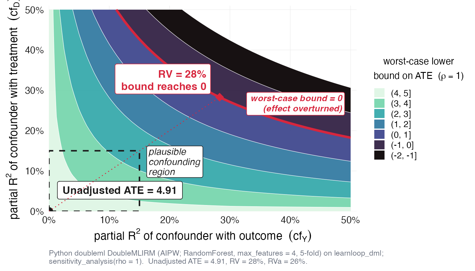
Across the plausible region the bound stays positive — overturning the effect needs a confounder about twice as strong as everything we measured.

The AIPW/IRM ATE (DoubleMLIRM): \(cf_d\) is the Riesz-norm dial. A PLR/PLIV effect would give the plain-sensemakr version.

Read the contour like the S06 sensemakr plot. The origin is the unadjusted DML estimate (≈ 4.9). Moving out along the axes, an ever-stronger confounder erodes the bound; the highlighted contour is where the lower bound hits zero. The robustness value is how far you have to travel to get there — here RV = 28%, about twice the ~15% the observed covariates explain, so overturning the effect needs a confounder roughly twice as strong as everything we measured. Robust, but with a ~2× margin — not an enormous one. Pair this with the named industry use case (Booking.com) in the notes: estimate, then stress-test, before acting. Provenance: Python doubleml DoubleMLIRM (AIPW, score = ATE; RandomForest, n_estimators = 500, max_features = 4, 5-fold) on learnloop_dml; sensitivity_analysis(rho = 1, worst case). Unadjusted ATE = 4.91; at cf_Y = cf_D = 3%, bound = 4.46; RV = 28% (bound → 0), RVa = 26% (estimate → insignificant at 5%).

Recap: one recipe, two ingredients, honest intervals

• FWL with a machine: partial \(X\) out of \(Y\) and \(D\) with any ML learner, then read the slope.
• Orthogonality kills regularization bias; cross-fitting kills overfitting bias — together they restore the \(\sqrt{n}\), normal CI.
• One score per estimand: PLR (constant effect), AIPW/IRM (doubly-robust ATE), IIVM (LATE).
• DML solves estimation, not identification — so always stress-test unconfoundedness.

Next week (S09): stop averaging the score \(\psi_i\) and start projecting it on \(X\) — heterogeneous effects \(\tau(x)\), meta-learners, causal forests. DML also powers DiD in Part V. (Chang 2020)

Tie the bow. The four bullets are the takeaways; if a student remembers only these, they can use DML responsibly. End on the hand-off: the per-unit AIPW score we named in Act 4 is the seed of next week’s heterogeneity methods — averaging gives the ATE, projecting gives tau(x). And flag that the same orthogonal-score logic reappears in Part V for difference-in-differences. Close on Knaus’s maxim one more time: DML is a powerful estimator, not a substitute for a credible identification argument.

References

Ahrens, Achim, Christian B. Hansen, Mark E. Schaffer, and Thomas Wiemann. 2025. “Model Averaging and Double Machine Learning.” Journal of Applied Econometrics 40 (3): 249–69. https://doi.org/10.1002/jae.3103.

Ballinari, Daniele, and Nora Bearth. 2024. “Improving the Finite Sample Estimation of Average Treatment Effects Using Double/Debiased Machine Learning with Propensity Score Calibration.” https://arxiv.org/abs/2409.04874.

Bang, Heejung, and James M. Robins. 2005. “Doubly Robust Estimation in Missing Data and Causal Inference Models.” Biometrics 61 (4): 962–73. https://doi.org/10.1111/j.1541-0420.2005.00377.x.

Chang, Neng-Chieh. 2020. “Double/Debiased Machine Learning for Difference-in-Differences Models.” The Econometrics Journal 23 (2): 177–91. https://doi.org/10.1093/ectj/utaa001.

Chernozhukov, Victor, Denis Chetverikov, Mert Demirer, Esther Duflo, Christian Hansen, Whitney Newey, and James Robins. 2018. “Double/Debiased Machine Learning for Treatment and Structural Parameters.” The Econometrics Journal 21 (1): C1–68. https://doi.org/10.1111/ectj.12097.

Chernozhukov, Victor, Carlos Cinelli, Whitney K. Newey, Amit Sharma, and Vasilis Syrgkanis. 2026. “Long Story Short: Omitted Variable Bias in Causal Machine Learning.” Review of Economics and Statistics, 1–45. https://doi.org/10.1162/rest.a.1705.

Chernozhukov, Victor, Whitney K. Newey, Víctor Quintas-Martínez, and Vasilis Syrgkanis. 2021. “Automatic Debiased Machine Learning via Riesz Regression.” https://arxiv.org/abs/2104.14737.

Chernozhukov, Victor, Whitney K. Newey, and Rahul Singh. 2022. “Automatic Debiased Machine Learning of Causal and Structural Effects.” Econometrica 90 (3): 967–1027. https://doi.org/10.3982/ECTA18515.

Cinelli, Carlos, and Chad Hazlett. 2020. “Making Sense of Sensitivity: Extending Omitted Variable Bias.” Journal of the Royal Statistical Society: Series B 82 (1): 39–67. https://doi.org/10.1111/rssb.12348.

Crump, Richard K., V. Joseph Hotz, Guido W. Imbens, and Oscar A. Mitnik. 2009. “Dealing with Limited Overlap in Estimation of Average Treatment Effects.” Biometrika 96 (1): 187–99. https://doi.org/10.1093/biomet/asn055.

Frisch, Ragnar, and Frederick V. Waugh. 1933. “Partial Time Regressions as Compared with Individual Trends.” Econometrica 1 (4): 387–401. https://doi.org/10.2307/1907330.

Lovell, Michael C. 1963. “Seasonal Adjustment of Economic Time Series and Multiple Regression Analysis.” Journal of the American Statistical Association 58 (304): 993–1010. https://doi.org/10.1080/01621459.1963.10480682.

Robins, James M., Andrea Rotnitzky, and Lue Ping Zhao. 1994. “Estimation of Regression Coefficients When Some Regressors Are Not Always Observed.” Journal of the American Statistical Association 89 (427): 846–66. https://doi.org/10.1080/01621459.1994.10476818.

Robinson, Peter M. 1988. “Root-N-Consistent Semiparametric Regression.” Econometrica 56 (4): 931–54. https://doi.org/10.2307/1912705.

Thank you for your attention!
	www.startupengineer.io/team/ihl/ christoph-ihl christophihl