library(readr); library(dplyr); library(fixest)

iv <- read_csv(here::here("materials", "data", "learnloop_iv.csv"))

# (a) Naive: regress exam_score on whether the lesson was completed.
#     No controls at all. HC1 (heteroskedasticity-robust) SE.
m_naive <- # ___ YOUR CODE: feols(exam_score ~ completed, data = iv, vcov = "hetero")

# (b) "Kitchen sink": adjust for the RECOMMENDATION (lesson_rec) plus EVERY observed
#     covariate. If selection-on-observables held, this would be unbiased.
m_adj <- # ___ YOUR CODE: feols(exam_score ~ completed + lesson_rec + age + prior_courses +
         #   baseline_score + gender + region + device + track,
         #   data = iv, vcov = "hetero")

# Print both 'completed' coefficients side by side.
# ___ YOUR CODE: coef(m_naive)["completed"]; coef(m_adj)["completed"]

# (c) DAG (optional to draw, required to state in words). Declare the structure:
#     X -> lesson_rec -> exam_score   (algorithm's recommend decision, OBSERVED)
#     reminder -> completed           (random study reminder, the future instrument)
#     u -> completed ,  u -> exam_score  (student MOTIVATION, UNOBSERVED confounder)
#     completed -> exam_score         (the causal effect we want, true tau = 6)
library(dagitty)
g <- # ___ YOUR CODE: dagitty('dag {
     #   u [unobserved]
     #   X -> lesson_rec -> exam_score ; reminder -> completed
     #   u -> completed ; u -> exam_score ; completed -> exam_score ; lesson_rec -> completed
     # }')
# adjustmentSets(g, exposure = "completed", outcome = "exam_score") # which backdoor can X close?10 Session 7: Instrumental Variable Designs
10.1 Lecture Slides
10.2 Overview
This session opens the unobserved-confounding half of Part III. S06 assumed every confounder was measured: condition on \(\mathbf{X}\) and treatment is as-good-as-random. S07 abandons that bet. When an unmeasured \(u\) drives both treatment and outcome — for our running FitLife app, the user’s latent motivation drives both whether a notification is opened (\(D\)) and subsequent engagement (\(Y\)) — no adjustment set can close the backdoor. The fix is not a better estimator but a better source of variation: a slice of \(D\) that is unrelated to \(u\).
The session develops one intuition through two devices. An instrument \(Z\) harvests exogenous variation from a quasi-random nudge (the randomized pop-up reminder); a regression discontinuity harvests it from a quasi-random cutoff. We build the Wald estimand and 2SLS, confront the central dichotomy — under heterogeneous effects IV identifies a Local Average Treatment Effect on compliers, not the ATE — and then the credibility threats: weak instruments (first-stage \(F\), the effective \(F\), the Lee et al. (2022) honest-inference threshold, and Anderson–Rubin intervals). We tour the design family tech teams actually use — lotteries and randomized encouragement, natural experiments, judge/examiner leniency, and Bartik / shift-share exposure — and close with RDD, where fuzzy RDD is literally a local IV.
Three forward-pointers: S08 (double machine learning, when \(\mathbf{X}\) is high-dimensional), S09 (treatment-effect heterogeneity), and the panel-data designs of Part V. The PBL works a synthetic online-learning encouragement design (the “LearnLoop” platform) end to end as a parallel worked example, and Assignment III then applies the same toolkit to the FitLife app, bridging S06 and S07 on one dataset. The quantitative anchors in the sections below refer to that online-learning lab; the FitLife framing above is the conceptual setup you will carry into the assignment.
10.3 Lecture Notes
10.3.1 Exogenous variation — the shared idea behind IV and RDD
10.3.1.1 When backdoor adjustment runs out: find a source of randomness
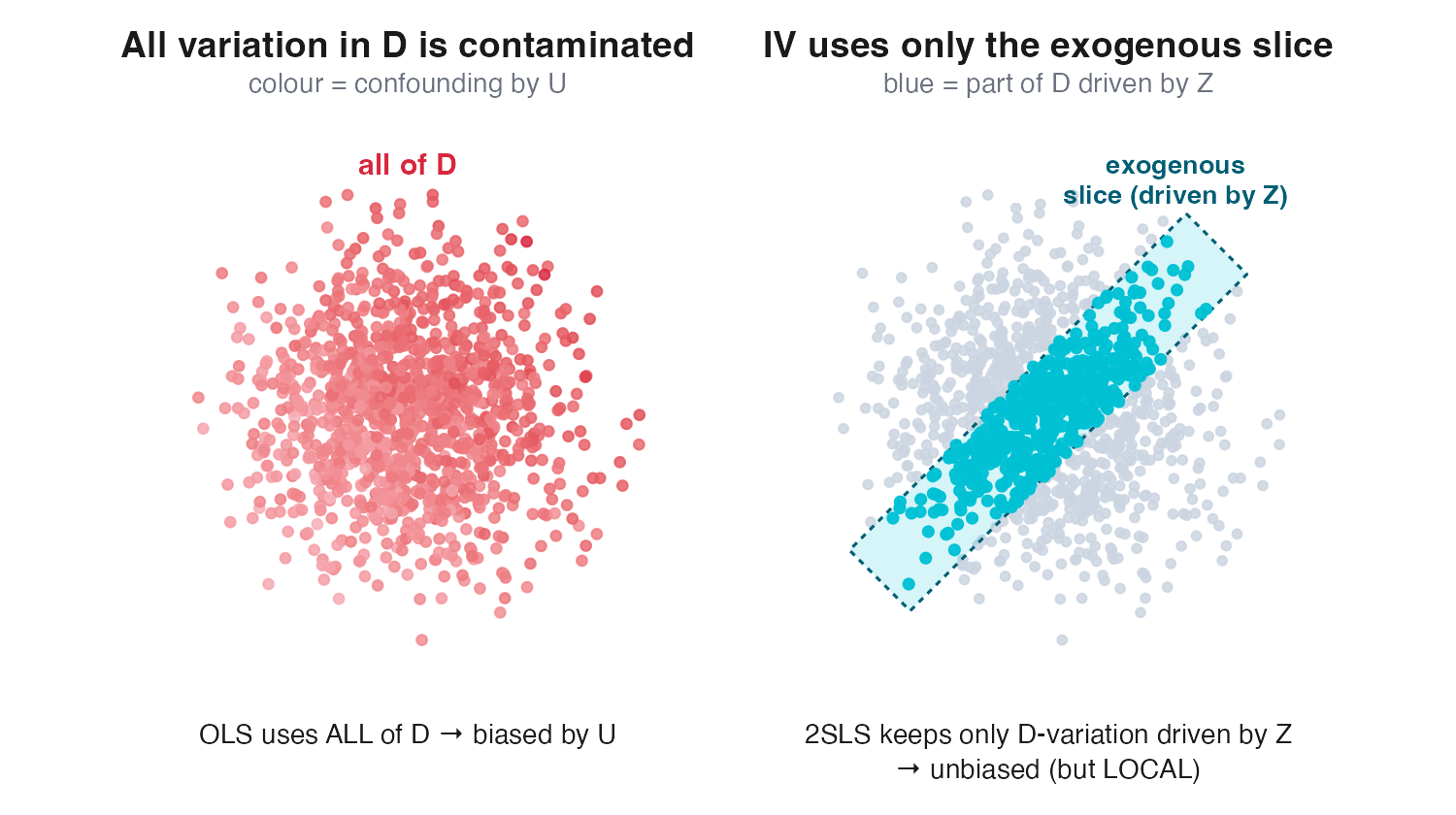
S06 closed by admitting that selection-on-observables fails whenever an unobserved confounder \(u\) drives both \(D\) and \(Y\) — for FitLife, the user’s latent motivation drives both whether a notification gets opened (\(D\)) and downstream engagement (\(Y\)). FitLife has two treatments: the algorithm’s SEND decision D_sent is confounded only by observed \(\mathbf{X}\), so S06 selection-on-observables identifies its effect, whereas the user’s opening choice D_opened is confounded by the unobserved \(u\), so S06 fails and we need IV — which is why opening is the harder problem and the focus of S07. No control set \(\mathbf{X}\) can block a path through a variable you never measured. The S06 premise is the formally untestable unconfoundedness statement \(D \perp \{Y(0), Y(1)\} \mid \mathbf{X}\), and by Manski’s Law of Decreasing Credibility (Manski 2003) sensitivity analysis only bounds how large an unobserved \(u\) would have to be — it never tests the assumption. The S07 move is to stop adjusting and instead locate an exogenous source of variation in \(D\) that is as good as randomly assigned. Both designs in this session are instances of one idea: isolate a slice of \(D\) that has no backdoor into \(Y\), and read the effect off that slice. Either way the design discards almost all of the variation in \(D\), keeping only the thin exogenous sliver the instrument (or cutoff) moves — which is why IV is far noisier than OLS, foreshadowing the weak-instrument precision cost. One warning worth planting now: both yield only a local effect — a LATE, or an effect at the cutoff — never a population ATE (the single most common student error).
10.3.1.2 The instrument DAG and the three core assumptions
An instrument \(Z\) (here: a randomly fired pop-up reminder) affects the outcome \(Y\) only through the treatment \(D\). In product terms this is an encouragement design — randomizing a nudge to adopt a feature you cannot withhold (Spotify’s template for feature-effect measurement, Elbers (2023)). The estimand of interest is \(\tau\), the effect of opening a notification on engagement.
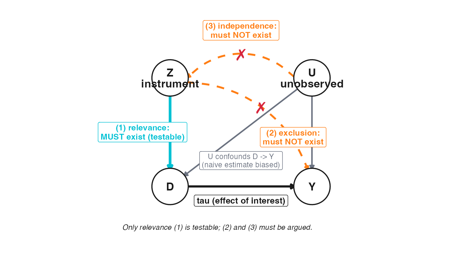
Identification rests on three assumptions, read directly off the DAG \(Z \to D \to Y\) with \(u \to D\), \(u \to Y\) but no \(u \to Z\) and no \(Z \to Y\):
- Relevance: \(\text{Cov}(Z, D \mid \mathbf{X}) \neq 0\) — the instrument actually moves treatment. Testable (the first stage).
- Independence (exogeneity / “as good as random”): \(Z \perp u \mid \mathbf{X}\) — the instrument is unconfounded with the unobservable. Untestable (it concerns \(u\)).
- Exclusion: \(Z\) affects \(Y\) only through \(D\), with no direct arrow \(Z \to Y\). Untestable, and a substantive, not a statistical, claim (Angrist, Imbens, and Rubin 1996).
The clean split: only relevance is checkable in the data. Independence and exclusion are defended by design and argument, which is why a credible instrument needs a credible story, not just a large F-statistic. The slides call this the strangeness principle: if a smart layperson finds \(Z\)’s link to \(Y\) puzzling — the only conceivable channel being \(D\) — that puzzlement is itself the exclusion evidence.
10.3.1.3 Monotonicity and the fourth assumption
For a binary instrument and treatment, adding monotonicity — no “defiers”, i.e. nobody does the opposite of what the instrument encourages — lets us interpret what IV recovers (Imbens and Angrist 1994). Formally, the encouragement weakly pushes everyone the same direction: \(D_i(Z=1) \geq D_i(Z=0)\) for all \(i\). Writing each type by its potential treatments \((D_i(Z=1), D_i(Z=0))\), monotonicity partitions the population into always-takers \((1,1)\), never-takers \((0,0)\), and compliers \((1,0)\), ruling out the fourth type, the defier \((0,1)\). It is partially refutable (negative first stages in subgroups are a red flag) but in general untestable.
10.3.2 From the Wald estimand to the LATE
10.3.2.1 The Wald estimand — reduced form over first stage
With a single binary instrument and no covariates — and, for now, a single effect \(\tau\) shared by everyone — the IV estimate is the Wald ratio: the reduced-form effect of the nudge on the outcome (\(Z \to Y\)) divided by the first-stage effect of the nudge on take-up (\(Z \to D\)),
\[\hat\tau_{\text{Wald}} = \frac{\text{reduced form}}{\text{first stage}} = \frac{\mathbb{E}(Y \mid Z=1) - \mathbb{E}(Y \mid Z=0)}{\mathbb{E}(D \mid Z=1) - \mathbb{E}(D \mid Z=0)}.\]
In the lab’s online-learning design the reduced form on the exam score is \(\approx 1.07\) and the first stage is \(\approx 0.180\), so \(\hat\tau_{\text{Wald}} \approx 1.07 / 0.180 \approx 6.0\) — in the neighbourhood of the true per-completion effect of \(6\), with the covariate-adjusted 2SLS below landing closer still. The intuition is rise-over-run: the nudge shifts completion by about \(18\%\), and with a single constant effect that shift carries straight through to the exam score, so dividing the reduced-form lift by the first-stage shift recovers the per-completion effect. (We hold the ITT / complier-share reading of this same ratio until heterogeneous effects, where dropping homogeneity makes those terms necessary.)
10.3.2.2 Two-stage least squares with covariates
Equivalently, the same estimand is the covariance ratio \(\tau = \operatorname{Cov}(Y,Z)/\operatorname{Cov}(D,Z)\); this form is what generalizes the binary difference-in-means to continuous instruments and is exactly what 2SLS computes. 2SLS generalizes the Wald ratio to continuous treatments and multiple covariates (Angrist and Pischke 2015). Stage one projects \(D\) on \(Z\) and the controls \(\mathbf{X}\) (crucially including lesson_rec, the algorithm’s recommendation); stage two regresses \(Y\) on the fitted \(\hat D\) and the same controls. Mechanically, 2SLS replaces the endogenous \(D\) with the part of it that is explained by exogenous \(Z\) — discarding exactly the variation correlated with \(u\). Never run the two stages by hand (regress \(D\) on \(Z\), then \(Y\) on the fitted \(\hat D\)): the point estimate is right, but the second-stage standard errors are too small because stage two treats \(\hat D\) as observed data rather than an estimated quantity — a common, silent bug. Always call a dedicated IV routine (R ivreg / fixest::feols, Python IV2SLS / DoubleML), which propagates first-stage uncertainty, and cluster the standard errors at the level of assignment. With lesson_rec and the demographic controls in both stages, the lab’s 2SLS estimate is \(\approx 6.1\), close to the truth of \(6\) and far below the naive OLS of \(\approx 8.2\) (and the still-biased \(\approx 7.4\) from regression on observables alone).
10.3.2.3 Homogeneous vs. heterogeneous effects, and why IV recovers a LATE
If the treatment effect is homogeneous (constant \(\tau\) for everyone), IV recovers that single \(\tau\) and the choice of instrument is innocuous. Under realistic heterogeneity, IV alone cannot nonparametrically identify the population ATE — relevance, independence, and exclusion are not enough; you recover only an average over compliers, and only once you add monotonicity do the three core assumptions identify the Local Average Treatment Effect (LATE; also the complier average causal effect, CACE) — the average effect for compliers only (Imbens and Angrist 1994):
\[\tau_{\text{LATE}} = \mathbb{E}\bigl[Y(1) - Y(0) \mid \text{complier}\bigr].\]
Read against the Wald ratio, dropping homogeneity simply re-labels the same two pieces: the reduced-form numerator is now the intention-to-treat (ITT) effect — the effect of offering the nudge, averaged over compliers and the unmoved alike — and the first-stage denominator is the complier share, so the identical ratio now reads \(\text{LATE} = \text{ITT} / \text{complier share}\). A LATE rests on five assumptions: SUTVA (no interference, one version of treatment), Independence (\(u \not\to Z\)), Exclusion (no direct \(Z \to Y\)), Relevance (\(Z\) moves \(D\)), and Monotonicity (no defiers). Always-takers and never-takers contribute nothing, because the instrument never changes their treatment status, so the data carry no counterfactual for them; and because each observed \((Z, D)\) cell still mixes two unobserved types, it is monotonicity — ruling out defiers — that leaves only compliers in the ratio.
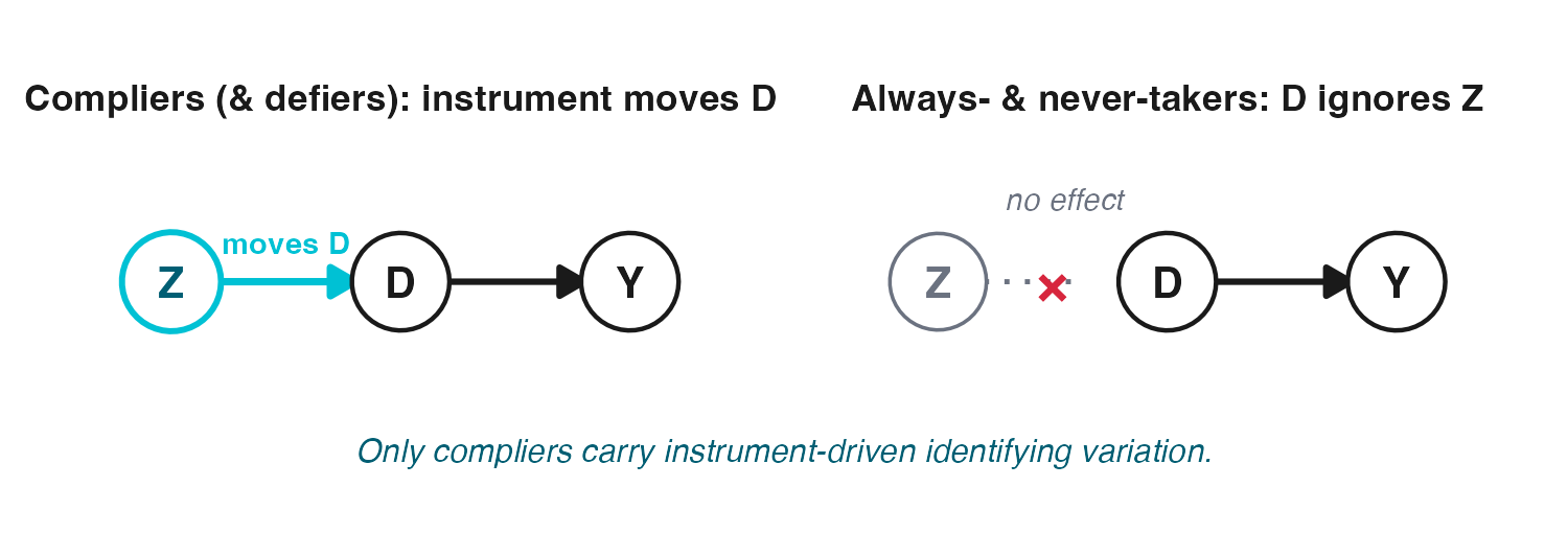
The estimand is defined by the instrument: a different \(Z\) moves a different complier subpopulation and recovers a different LATE.
10.3.2.4 ITT vs. LATE — two questions, two answers
The ITT answers a policy question: what happens to engagement if we deploy the reminder to everyone, compliers and non-compliers alike? The LATE answers a mechanism question: how much does actually opening a notification raise engagement, among those the reminder can sway? The Wald denominator is the bridge: \(\text{LATE} = \text{ITT} / (\text{complier share})\), so a small first stage inflates the LATE relative to the ITT. Reporting both, and naming the complier group, is the standard of honest IV practice (Angrist, Imbens, and Rubin 1996).
10.3.3 Weak instruments
10.3.3.1 The first-stage F and why “F > 10” is a dangerous habit
When the instrument barely moves treatment, the first-stage denominator is near zero and 2SLS becomes badly biased — toward OLS — with severely distorted standard errors. The relative bias of 2SLS toward the OLS plim is approximately \(\tfrac{1}{F+1}\) (Bound, Jaeger, and Baker 1995), so at \(F\to 0\) the instrument buys nothing; and the “false precision” of the reported SE means under-coverage — a nominal \(95\%\) conventional CI covers the truth far less than \(95\%\) of the time when the instrument is weak. The classic diagnostic is the partial first-stage F-statistic on the excluded instrument(s) — covariates partialled out by Frisch–Waugh–Lovell, not the overall regression F, which strong controls can inflate enough to mask a weak instrument; the Staiger and Stock (1997) / Stock and Yogo (2005) rule of thumb \(F > 10\) became the field default. In the just-identified case the first-stage F is simply the squared \(t\) on the \(D\)-on-\(Z\) coefficient, so a weak instrument is imprecise, not necessarily small. The strong reminder instrument in the lab has \(F \approx 376\), comfortably clearing any threshold. A Monte-Carlo picture makes the decay tangible: as the first stage weakens, the 2SLS sampling distribution simultaneously drifts toward the (biased) OLS plim and fattens in the tails — the bias and the lost precision worsen together as \(F\) falls; Exercise 4 in the lab reproduces this by stepping the first-stage strength down.
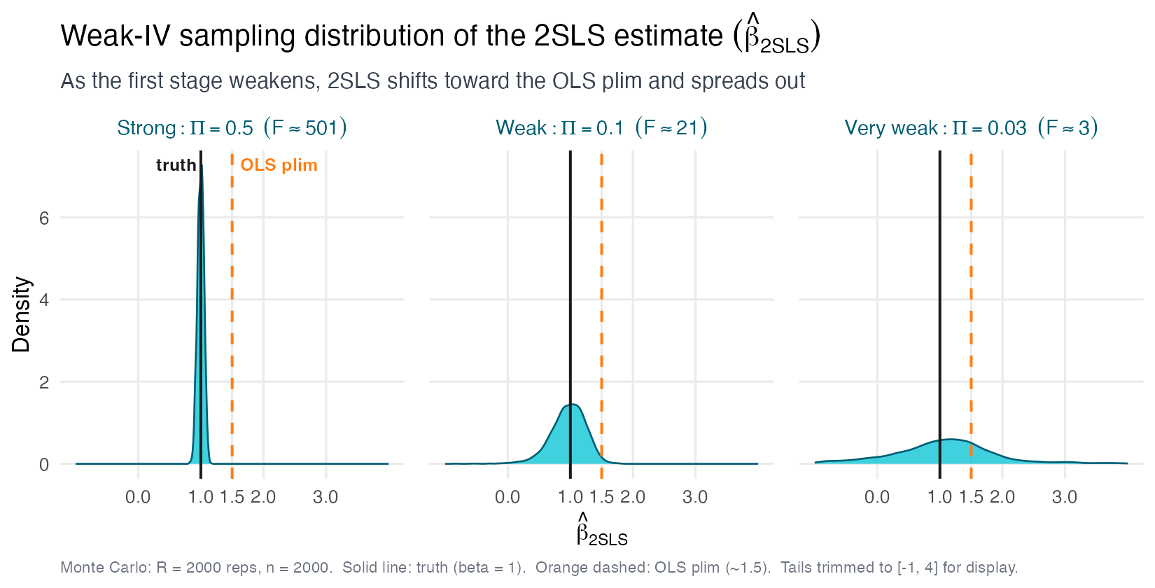
The danger: the weak reminder instrument in the lab has \(F \approx 10.8\) — it passes the naive \(F > 10\) screen — yet its 2SLS estimate (\(\approx 7.6\)) carries a conventional t-CI of \(\approx [-0.4,\, 15.6]\) that spans zero.
10.3.3.2 The effective F and the Lee et al. threshold
Two refinements supersede the naive rule. With non-homoskedastic or clustered errors, use the effective F-statistic (Montiel Olea and Pflueger 2013) rather than the textbook first-stage F. (The homoskedastic textbook F is the Cragg–Donald F, and its cluster-robust counterpart the Kleibergen–Paap rk Wald F (Kleibergen and Paap 2006) — what ivreg2 / ivreghdfe print; the effective F is a distinct robust statistic judged against its own critical value, not \(10\), though with a single instrument all three coincide.) And Lee et al. (2022) show that to keep a nominal \(5\%\) 2SLS t-test honest, the required first-stage F is not \(10\) but roughly \(\mathbf{104.7}\) — an order of magnitude larger. Rather than a single pass/fail cutoff, Lee et al. (2022) also supply a smooth standard-error inflation factor indexed by the observed first-stage F — the tF procedure — largest for weak first stages and shrinking to the usual \(1.96\) critical value only once \(F\) reaches \(104.7\), so weak-IV adjustment is a continuous correction rather than a cliff-edge pass/fail. By this standard the weak instrument in the lab (\(F \approx 10.8\)) is decisively weak, even though it survives the folklore cutoff. The practical lesson: the \(F>10\) rule licenses overconfident inference.
10.3.3.3 Anderson–Rubin — inference that survives weak instruments
The Anderson–Rubin test (Anderson and Rubin 1949) sidesteps the problem entirely: it inverts a test on the reduced form and is valid regardless of instrument strength (Andrews, Stock, and Sun 2019). Concretely, for each candidate \(\beta_0\) regress \((Y - \beta_0 D)\) on \(Z\) and the controls; the AR confidence set is every \(\beta_0\) for which the coefficient on \(Z\) is insignificant (\(|t_Z| < 1.96\)). In the just-identified case — the typical encouragement design — AR is the most powerful weak-IV-robust test, so defaulting to it costs no power. For the weak instrument in the lab the AR \(95\%\) CI is \(\approx [-2.2,\, 17.6]\) — wider than the t-interval and honestly admitting how little the data pin down. When instruments may be weak, report AR (or a weak-IV-robust analogue), not the 2SLS t-CI.
10.3.4 The design family — where exogenous variation comes from
10.3.4.1 Lotteries and explicit randomization
The cleanest instruments are literal random draws. Oversubscribed school admissions, randomized waitlists, and randomized encouragement assign \(Z\) by lottery, so independence holds by construction and only exclusion remains arguable. Tech example: a feature is rolled out to a random subset, but adoption is voluntary — the random assignment instruments for actual use, exactly the lab’s study reminder \(Z\) for lesson completion \(D\).
10.3.4.2 Natural experiments and encouragement designs
When no lottery exists, an encouragement design nudges a random subgroup toward treatment without forcing it — the canonical setting for (Angrist, Imbens, and Rubin 1996)’s LATE framework. More broadly, natural experiments exploit quasi-random administrative or institutional variation (policy thresholds, arbitrary timing, geographic discontinuities). Tech example: staggered server-side rollout where the order of regions is plausibly unrelated to outcomes instruments for early exposure to a new ranking model — or recommender noise, where a ranker’s random jitter in what gets surfaced instruments item exposure (Sharma, Hofman, and Watts 2015), the one platform-native case where the system itself emits the randomness. “As good as random” is a claim, not a fact: defend it with balance tests, pre-trends, and the adversary’s question — what else changed at the same moment? — and remember it holds only conditional on \(\mathbf{X}\).
10.3.4.3 Judge / examiner leniency
When cases are assigned as good as randomly to decision-makers who differ in strictness, the assigned examiner’s average leniency instruments for the individual decision. Build each unit’s instrument from the assigned examiner’s leniency computed leaving out case \(i\)’s own decision, demeaned within the office-by-time cell, so only relative strictness — not caseload composition — drives \(Z\): \(Z_i = \bar{D}_{-i,\,j(i)} - \bar{D}_{\text{cell}(i)}\). Including case \(i\)’s own decision inside its own instrument mechanically fakes a first stage — the single most common implementation bug. The fine print: exclusion can fail through side-channels (a strict examiner may move \(Y\) by routes other than the focal \(D\), e.g. ordering rehab programs); monotonicity is itself testable (Frandsen, Lefgren, and Leslie 2023); and with many judges each contributing little, 2SLS suffers many-weak-instrument bias toward OLS, so use a jackknife-IV / UJIVE estimator and cluster standard errors at the assignment unit (Chyn, Frandsen, and Leslie 2025). Tech example: support tickets routed round-robin to moderators of varying strictness — the assigned moderator’s baseline ban rate instruments for whether a given account is actioned, identifying the effect of enforcement on user retention. The same machinery answers two distinct managerial questions: Q1 — the effect of the decision on the outcome (the 2SLS use here), and Q2 — an audit for bias at the margin across decision-makers via the outcome test (Dobbie et al. 2021; Arnold, Dobbie, and Yang 2018).
10.3.4.4 Bartik / shift-share instruments
Shift-share (Bartik) instruments combine common “shifts” with pre-existing local “shares” to manufacture exogenous variation in a regional treatment, \(Z_\ell = \sum_k s_{\ell k}\, g_k\) (Bartik 1991).
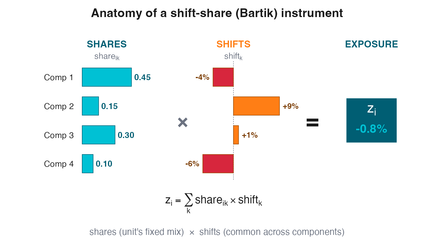
Identification leans on the exogeneity of either the shares or the shifts: either the shares are as-good-as-random (Goldsmith-Pinkham, Sorkin, and Swift 2020) (identification strength scales with the number of regions) or the shifts are (Borusyak, Hull, and Jaravel 2022) (the effective sample size is the number of shifts, often alarmingly small) — reserve “shock” for a shift you specifically claim is exogenous. Rotemberg weights reveal which few industries actually drive the estimate, so you must declare which story you rely on: which side carries identification is regime-conditional — a handful of high-weight shares when the shifts are few (defend those shares), or the shifts themselves when they are many (the shares may even be endogenous), never an automatic default to the shares. Tech example: a platform’s exposure to an industry-wide demand shift, weighted by each market’s historical seller mix, instruments for local marketplace volume when estimating the effect of volume on take-rate. The live tech template is the robot design — predicted exposure (1990 industry shares \(\times\) European robot adoption, Acemoglu and Restrepo (2020)) instruments actual US robot exposure, with the AI analogue swapping industry shares for occupation shares. Watch the standard errors: naive and even state-clustered SEs understate uncertainty because regions with similar industry shares load on the same national shifts — the correlation lives in exposure (share) space, not geography, so geographic clustering fails. Use exposure-robust AKM/AKM0 standard errors (Adão, Kolesár, and Morales 2019) (e.g. the ShiftShareSE package); as Exercise 8 in the lab shows, naive 95% CIs can cover the truth only about 60% of the time.
10.3.5 Regression discontinuity
10.3.5.1 Sharp and fuzzy designs
An RDD exploits a threshold rule: treatment switches at a cutoff \(c\) of a running variable \(X_{\text{run}}\). In a sharp design treatment is a deterministic step, \(D = \mathbf{1}\{X_{\text{run}} \geq c\}\); in a fuzzy design crossing the cutoff only shifts the probability of treatment (Hahn, Todd, and Van der Klaauw 2001).
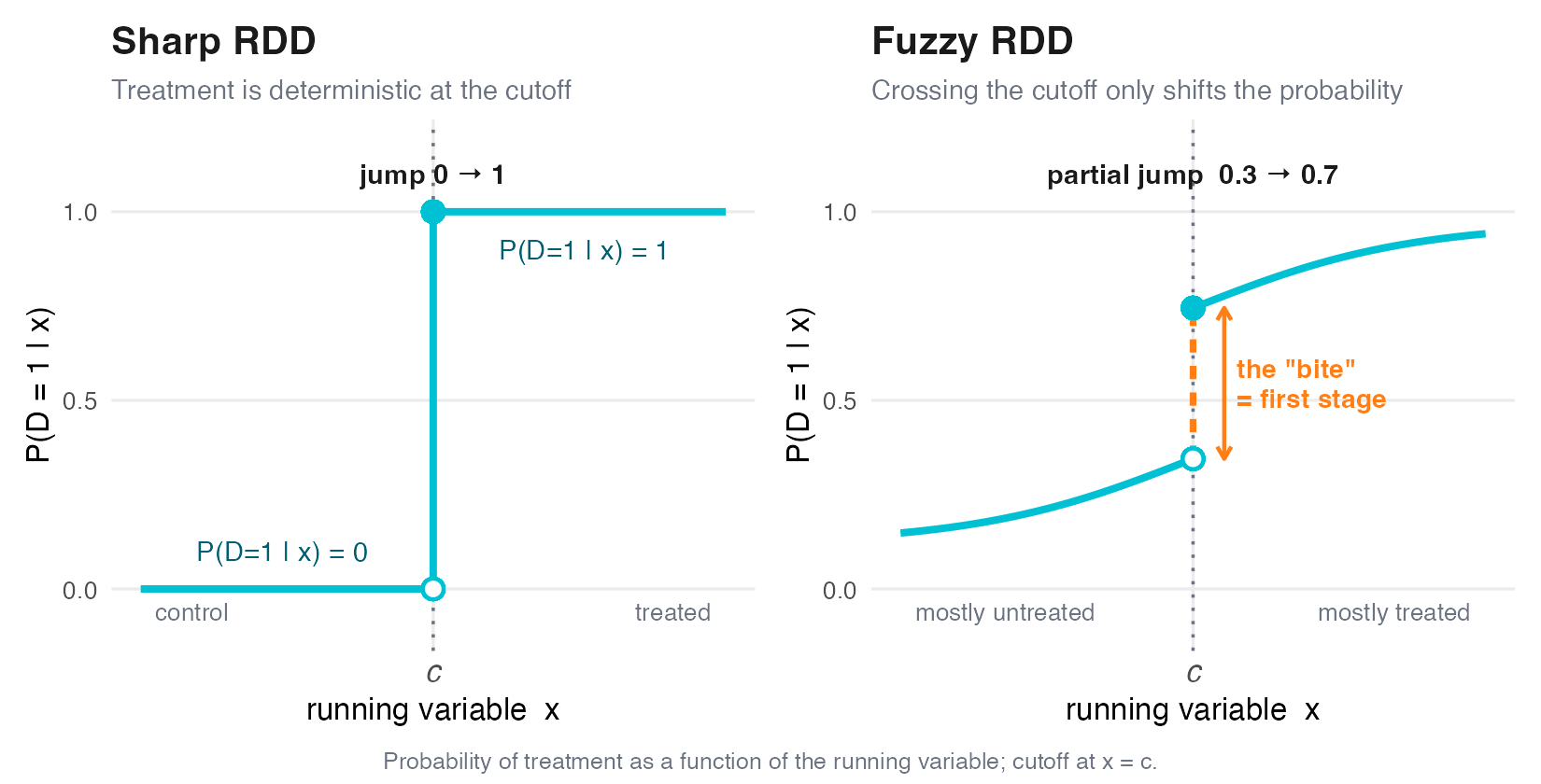
The identifying logic is local randomization: units just below and just above \(c\) are comparable on everything except their treatment-relevant position, so the discontinuity in \(Y\) at \(c\) is causal. The lab’s RDD data are fuzzy — crossing the cutoff (\(c = 60\) on the course-progress score \(X_{\text{run}}\)) raises the treatment probability by a “bite” of only \(\approx 0.47\), not to \(1\). The same diagnostic classifies real thresholds: mechanical gates (tier auto-enrolment, auction reserves, search-rank cutoffs) are sharp, while discretionary or opt-in gates (credit approval, promo redemption, fraud review) are fuzzy.
10.3.5.2 Fuzzy RDD is a local instrumental-variables estimator
The two halves of this session meet here: a fuzzy RDD is IV applied locally at the cutoff. The threshold indicator \(\mathbf{1}\{X_{\text{run}} \geq c\}\) plays the role of the instrument \(Z\), and the fuzzy-RDD estimate is a local Wald ratio — the jump in \(Y\) divided by the jump in \(P(D)\),
\[\tau_{\text{fuzzy}} = \frac{\lim_{x \downarrow c}\mathbb{E}(Y\mid X_{\text{run}}=x) - \lim_{x \uparrow c}\mathbb{E}(Y\mid X_{\text{run}}=x)}{\lim_{x \downarrow c}\mathbb{E}(D\mid X_{\text{run}}=x) - \lim_{x \uparrow c}\mathbb{E}(D\mid X_{\text{run}}=x)}.\]
Like IV, it recovers a LATE — the effect for compliers at the cutoff (sharp RDD is just the special case where this first-stage jump equals \(1\)). This makes RDD doubly local: beyond the complier sense, it is also local in the covariate sense — the effect is identified only for units near \(c\), and extrapolating it to a different threshold (say, from a \(60\%\) progress gate to a \(90\%\) one — different students, different stakes) is an assumption, not a finding. The lab’s fuzzy LATE is \(\approx 6.03\) with robust CI \(\approx [4.8,\, 8.2]\), reassuringly close to the encouragement LATE of \(\approx 6.1\) from the Wald estimand to the LATE: two designs, two complier groups, the same underlying effect.
10.3.5.3 Smoothness identifies; it does not estimate
The RDD assumption is continuity: all confounders, and the potential-outcome functions \(\mathbb{E}(Y(0)\mid X_{\text{run}})\) and \(\mathbb{E}(Y(1)\mid X_{\text{run}})\), vary smoothly through \(c\), so any jump in \(Y\) must be the treatment (Calonico, Cattaneo, and Titiunik 2014). But smoothness is an assumption about the true regression function — it does not license fitting a smooth high-order polynomial to estimate the jump. Gelman and Imbens (2019) show that global high-order polynomials produce noisy, artefactual discontinuities and weights nobody would choose deliberately. The estimator is therefore local linear regression on each side, inside a data-driven bandwidth (CCT \(\approx 10.8\) for the lab), not a quartic on the full support.
10.3.5.4 Validity checks: density continuity and covariate smoothness
An RDD is only as credible as its no-manipulation premise: if units can precisely sort across the cutoff, comparability breaks. The McCrary / rddensity test (McCrary 2008; Cattaneo, Jansson, and Ma 2020) checks for a discontinuity in the density of \(X_{\text{run}}\) at \(c\) — a spike on the treated side signals gaming. The lab passes cleanly (\(p \approx 0.47\), no detectable manipulation). Because running variables often heap at round numbers, a spurious density jump is checked with a donut-hole fit — drop the observations right at \(c\) and re-estimate. The complementary check: pre-treatment covariates (e.g. baseline_score) should be continuous at \(c\) — a placebo RDD on each should find no jump. A second falsification: re-run the same RDD at fake cutoffs \(c' \neq c\) where no treatment actually changes — a “jump” detected there signals a misspecified design.
10.3.5.5 Tooling and the reporting standard
The modern RDD toolkit is rdrobust (R and Python ports alike): rdrobust(Y, X_run, fuzzy = D, c = 50) returns the CCT-optimal bandwidth and robust bias-corrected confidence intervals, rdplot() produces the canonical binned-scatter-with-fit figure, and rddensity() runs the manipulation test (Calonico, Cattaneo, and Titiunik 2014; Cattaneo, Jansson, and Ma 2020). The credible RDD report bundles four artefacts: the rdplot, the robust point estimate and CI, the density test, and covariate-smoothness placebos — the discontinuity-design analogue of the balance table in S06 (Cunningham 2021).
10.4 Coding Lab
The lab works an online-learning encouragement design end to end on a synthetic dataset where the truth is known (effect of completing a recommended lesson on the exam score \(= +6\)). The setting is LearnLoop, a course platform: a learning-science team wants the causal effect of a student completing a recommended lesson, but completion is the student’s own choice. Each exercise gives a Scaffold with # ___ YOUR CODE placeholders in both R and Python; attempt it, then expand Show solution to compare.
Download the datasets: learnloop_iv.csv · learnloop_iv_weak.csv · learnloop_rdd.csv
10.4.1 Exercise 1 — Why OLS fails: the confounded encouragement setup (~20 min)
LearnLoop’s algorithm decides which students to recommend a lesson to (lesson_rec), but whether a student actually completes it (completed, our treatment of interest) is the student’s own choice. The learning-science team wants the causal effect of completing a recommended lesson on the end-of-unit exam score (exam_score). In this exercise you establish the problem: you will estimate the completion–exam relationship two ways — raw and fully adjusted for every observed covariate — and discover that even controlling for everything you can see leaves the estimate biased, because the thing that drives both completing and exam performance (a student’s underlying motivation u) is never recorded. This motivates the instrument in Exercise 2.
10.4.1.1 Scaffold
import pandas as pd
import statsmodels.formula.api as smf

iv = pd.read_csv("../../materials/data/learnloop_iv.csv")

# (a) Naive: exam_score on completed, no controls, HC1 robust SE.
m_naive = # ___ YOUR CODE: smf.ols("exam_score ~ completed", iv).fit(cov_type="HC1")

# (b) Kitchen sink: lesson_rec + every observed covariate (categoricals via C()).
m_adj = # ___ YOUR CODE: smf.ols(
        #   "exam_score ~ completed + lesson_rec + age + prior_courses + baseline_score"
        #   " + C(gender) + C(region) + C(device) + C(track)",
        #   iv).fit(cov_type="HC1")

# Print both 'completed' coefficients.
# ___ YOUR CODE: print(m_naive.params["completed"], m_adj.params["completed"])

# (c) State the DAG in words (see R tab): u -> completed and u -> exam_score is the
#     backdoor that NO observed X can block, because u is never recorded.
TipShow solution
library(readr); library(dplyr); library(fixest)

iv <- read_csv(here::here("materials", "data", "learnloop_iv.csv"),
               show_col_types = FALSE)

# (a) Naive OLS — no controls.
m_naive <- feols(exam_score ~ completed, data = iv, vcov = "hetero")

# (b) Kitchen-sink OLS — recommendation + every observed covariate.
m_adj <- feols(
  exam_score ~ completed + lesson_rec + age + prior_courses + baseline_score +
      gender + region + device + track,
  data = iv, vcov = "hetero")

cat("naive  completed coefficient:", round(coef(m_naive)["completed"], 3), "\n")  # ~8.19
naive completed coefficient: 8.187 cat("adjusted completed coefficient:", round(coef(m_adj)["completed"], 3), "\n") # ~7.44adjusted completed coefficient: 7.437 cat("true effect (by construction):", 6, "\n")true effect (by construction): 6 # (c) The DAG: X -> lesson_rec -> exam_score is observed; u -> completed, u -> exam_score
# is the backdoor; no observed adjustment set can close it because u is hidden.
suppressMessages(library(dagitty))
g <- dagitty('dag {
u [unobserved]
X -> lesson_rec
lesson_rec -> exam_score
lesson_rec -> completed
reminder -> completed
u -> completed
u -> exam_score
completed -> exam_score
}')
print(adjustmentSets(g, exposure = "completed", outcome = "exam_score"))import pandas as pd
import statsmodels.formula.api as smf
iv = pd.read_csv("../../materials/data/learnloop_iv.csv")
# (a) Naive OLS.
m_naive = smf.ols("exam_score ~ completed", iv).fit(cov_type="HC1")
# (b) Kitchen-sink OLS.
m_adj = smf.ols(
"exam_score ~ completed + lesson_rec + age + prior_courses + baseline_score"
" + C(gender) + C(region) + C(device) + C(track)",
iv).fit(cov_type="HC1")
print("naive completed coefficient:", round(m_naive.params["completed"], 3)) # ~8.19naive completed coefficient: 8.187print("adjusted completed coefficient:", round(m_adj.params["completed"], 3)) # ~7.44adjusted completed coefficient: 7.437print("true effect (by construction): 6")true effect (by construction): 6The naive regression returns roughly 8.2 — biased upward relative to the true effect of 6 (Angrist and Pischke 2015). The mechanism is selection: students who complete recommended lessons are the motivated ones, and motivated students would have scored higher anyway. Completion is a proxy for that motivation, so the raw coefficient pools the genuine treatment effect with a motivation premium.
The kitchen-sink regression — lesson_rec plus every observed covariate — drags the estimate down to about 7.4, closer but still above 6. This is the lesson of the exercise: adjustment is not a cure. Reading the DAG, conditioning on X (and on lesson_rec, which X causes) closes the back-door paths through observed variables like the algorithm’s recommendation, but it does nothing to the path completed ← u → exam_score. The student’s underlying motivation u drives both the decision to complete the lesson and subsequent exam performance, and u is never recorded, so it cannot enter any adjustment set — dagitty returns no valid set that uses only observed nodes. No amount of observed control closes a backdoor that runs through an unobserved variable (Cunningham 2021). The residual gap of ~1.4 is exactly that uncloseable path. Exercise 2 sidesteps it entirely by exploiting the random study reminder reminder, which affects exam_score only through completed and is independent of u.
10.4.2 Exercise 2 — Wald by hand, then 2SLS (~30 min)
With a valid instrument in hand, the LATE has a deceptively simple form: it is the intention-to-treat (ITT) effect of the reminder on the exam score, rescaled by the first-stage effect of the reminder on completion. You will first build this Wald ratio by hand from four group means on learnloop_iv.csv, then reproduce (and sharpen) it with covariate-adjusted 2SLS, and finally read off the first-stage \(F\) that tells you the instrument is strong. The deliverable is one ratio computed manually, one 2SLS coefficient, and one \(F\)-statistic — with a sentence on why all three agree with the true effect of 6.
10.4.2.1 Scaffold
library(readr); library(dplyr); library(fixest)
df <- read_csv(here::here("materials", "data", "learnloop_iv.csv"))

# (a) Wald by hand: ITT (reminder on exam_score) / first stage (reminder on completed),
#     ignoring covariates. Compute the four group means with dplyr.
itt        <- # ___ YOUR CODE: mean(exam_score | reminder==1) - mean(exam_score | reminder==0)
first_stage <- # ___ YOUR CODE: mean(completed | reminder==1) - mean(completed | reminder==0)
wald       <- # ___ YOUR CODE: itt / first_stage   # expect ≈ 1.07 / 0.180 ≈ 6.0

# (b) Covariate-adjusted 2SLS. fixest syntax: structural controls on the LHS of `|`,
#     the endogenous regressor and its instrument after it as  completed ~ reminder.
#     Controls = lesson_rec (the algorithm's RECOMMENDATION) + all baseline covariates.
iv <- # ___ YOUR CODE: feols(exam_score ~ lesson_rec + age + prior_courses + baseline_score +
      #                        gender + region + device + track | completed ~ reminder,
      #                        data = df, vcov = "hetero")
# summary(iv)   # the `fit_completed` row is the LATE; expect ≈ 6.1

# (c) First-stage strength. fitstat(., ~ ivf1) reports the (heteroskedasticity-robust)
#     first-stage F on the excluded instrument 'reminder'.
# ___ YOUR CODE: fitstat(iv, ~ ivf1)   # expect F ≈ 376

# (d) Cross-check the point estimate with a second engine (pick one):
#     estimatr::iv_robust(exam_score ~ lesson_rec + ... | lesson_rec + ... + reminder, data = df)  OR
#     AER::ivreg(exam_score ~ lesson_rec + ... + completed | lesson_rec + ... + reminder, data = df)
import pandas as pd, numpy as np
from linearmodels.iv import IV2SLS
df = pd.read_csv("../../materials/data/learnloop_iv.csv")
# (a) Wald by hand with numpy: ITT / first stage, ignoring covariates.
itt = # ___ YOUR CODE: df.loc[df.reminder==1,"exam_score"].mean() - df.loc[df.reminder==0,"exam_score"].mean()
first_stage = # ___ YOUR CODE: df.loc[df.reminder==1,"completed"].mean() - df.loc[df.reminder==0,"completed"].mean()
wald = # ___ YOUR CODE: itt / first_stage # expect ≈ 6.0
# (b) Covariate-adjusted 2SLS. linearmodels formula: the endogenous regressor and its
# instrument go in [completed ~ reminder]; everything else is an exogenous control.
m = # ___ YOUR CODE:
# IV2SLS.from_formula(
# "exam_score ~ 1 + lesson_rec + age + prior_courses + baseline_score + "
# "C(gender) + C(region) + C(device) + C(track) + [completed ~ reminder]",
# df).fit(cov_type="robust")
# print(m.params["completed"]) # the LATE; expect ≈ 6.1
# (c) First-stage strength: the F on 'reminder' lives in m.first_stage.diagnostics
# ___ YOUR CODE: print(m.first_stage.diagnostics) # expect F ≈ 376
TipShow solution
library(readr); library(dplyr); library(fixest)
df <- read_csv(here::here("materials", "data", "learnloop_iv.csv"))

# (a) Wald by hand --------------------------------------------------------
itt         <- mean(df$exam_score[df$reminder == 1]) - mean(df$exam_score[df$reminder == 0])
first_stage <- mean(df$completed[df$reminder == 1]) - mean(df$completed[df$reminder == 0])
wald        <- itt / first_stage
cat(sprintf("ITT = %.3f  | first stage = %.3f  | Wald LATE = %.2f\n",
            itt, first_stage, wald))
ITT = 1.072 | first stage = 0.180 | Wald LATE = 5.96# (b) Covariate-adjusted 2SLS ---------------------------------------------
iv <- feols(exam_score ~ lesson_rec + age + prior_courses + baseline_score +
gender + region + device + track | completed ~ reminder,
data = df, vcov = "hetero")
cat(sprintf("2SLS LATE (fit_completed) = %.2f\n", coef(iv)["fit_completed"]))2SLS LATE (fit_completed) = 6.07print(confint(iv)["fit_completed", ]) 2.5 % 97.5 %
fit_completed 4.696923 7.450022# (c) First-stage F on the excluded instrument 'reminder' ------------------
print(fitstat(iv, ~ ivf1))F-test (1st stage), completed: stat = 376.16, p < 2.2e-16, on 1 and 9,989 DoF.# (d) Cross-check with a second engine ------------------------------------
ivr <- estimatr::iv_robust(
exam_score ~ lesson_rec + age + prior_courses + baseline_score +
gender + region + device + track + completed |
lesson_rec + age + prior_courses + baseline_score +
gender + region + device + track + reminder,
data = df, se_type = "HC1")
cat(sprintf("iv_robust LATE (completed) = %.2f\n", coef(ivr)["completed"]))iv_robust LATE (completed) = 6.07import pandas as pd, numpy as np
from linearmodels.iv import IV2SLS
df = pd.read_csv("../../materials/data/learnloop_iv.csv")
# (a) Wald by hand
itt = df.loc[df.reminder == 1, "exam_score"].mean() - df.loc[df.reminder == 0, "exam_score"].mean()
first_stage = df.loc[df.reminder == 1, "completed"].mean() - df.loc[df.reminder == 0, "completed"].mean()
wald = itt / first_stage
print(f"ITT = {itt:.3f} | first stage = {first_stage:.3f} | Wald LATE = {wald:.2f}")ITT = 1.072 | first stage = 0.180 | Wald LATE = 5.96# (b) Covariate-adjusted 2SLS
m = IV2SLS.from_formula(
"exam_score ~ 1 + lesson_rec + age + prior_courses + baseline_score + "
"C(gender) + C(region) + C(device) + C(track) + [completed ~ reminder]",
df).fit(cov_type="robust")
print(f"2SLS LATE (completed) = {m.params['completed']:.2f}")2SLS LATE (completed) = 6.08print(m.conf_int().loc["completed"].round(2).to_dict()){'lower': 4.7, 'upper': 7.45}# (c) First-stage F on 'reminder'
print(m.first_stage.diagnostics[["f.stat", "f.pval"]].round(3)) f.stat f.pval
completed 378.722 0.0The two recipes tell the same story. The Wald ratio by hand is the ITT of the reminder on the exam score (\(\approx 1.07\)) divided by the share of students it actually nudges into completing (\(\approx 0.180\)), giving \(\approx 1.07 / 0.180 \approx 6.0\). This is the LATE among compliers — students who complete because the reminder fired — and the small denominator simply rescales the ITT up to a per-completion effect; it does not destabilise anything because the first stage is precisely estimated. Adding lesson_rec and the baseline covariates to 2SLS moves the estimate to \(\approx 6.1\), with a heteroskedasticity-robust CI comfortably away from zero, and the estimatr (or AER) cross-check returns the same number — confirming this is a real estimate, not an engine artefact (Imbens and Angrist 1994; Angrist, Imbens, and Rubin 1996).
That both quantities (hand-Wald \(6.0\), 2SLS \(6.1\)) bracket the true effect of 6 is exactly what the IV machinery promises when the instrument is valid: with a random reminder and monotone compliance, \(\text{ITT}/\text{first stage}\) identifies the complier average causal effect, and covariate adjustment trims sampling noise to pull the point estimate onto the truth. The first-stage \(F \approx 376\) is the green light: it sits far above the Stock–Yogo / rule-of-thumb threshold of 10, so weak-instrument bias is negligible and conventional 2SLS inference is trustworthy here (Staiger and Stock 1997; Stock and Yogo 2005) — a luxury Exercise 4 will deliberately take away. This LATE of \(\approx 6.1\) is also the natural benchmark for Exercise 5’s fuzzy-RDD estimate (\(\approx 6.0\)): two different identification strategies, two different complier populations, one consistent answer.
10.4.3 Exercise 3 — Compliers and the LATE interpretation (~20 min)
The 2SLS estimate from Exercise 2 is not the average effect of completing a lesson for everyone — it is the effect for compliers, the students who complete because the reminder nudged them. Here you will use the four (reminder, completed) cells to decompose the population into compliance types under monotonicity, profile who the compliers are on observed covariates \(X\), and contrast the intention-to-treat (ITT) effect of the reminder with the local average treatment effect (LATE) of completing. The deliverable is the three type shares, a bar chart, and a one-sentence statement of which population the LATE describes.
10.4.3.1 Scaffold
library(readr); library(dplyr); library(ggplot2)

iv <- read_csv(here::here("materials", "data", "learnloop_iv.csv"))

# (a) First stage by instrument arm: P(completed = 1 | reminder = z) in each cell.
shares <- iv |>
  group_by(reminder) |>
  summarise(p_done = mean(completed), .groups = "drop")  # ___ YOUR CODE: E[completed | reminder]

p_d1_z0 <- # ___ YOUR CODE: P(completed = 1 | reminder = 0)  -> always-takers
p_d1_z1 <- # ___ YOUR CODE: P(completed = 1 | reminder = 1)

# (b) Compliance-type shares under monotonicity (no defiers):
complier   <- # ___ YOUR CODE: p_d1_z1 - p_d1_z0   (the first-stage gap)
always     <- # ___ YOUR CODE: p_d1_z0
never      <- # ___ YOUR CODE: 1 - p_d1_z1

# (c) Profile WHO the compliers are. We cannot label individuals as compliers,
#     but Abadie's kappa weights recover the complier *distribution* of any X.
#     kappa = 1 - D(1 - Z)/(1 - P(Z=1|X)) - (1 - D)Z/P(Z=1|X).
pz <- predict(glm(reminder ~ age + prior_courses + baseline_score,
                  data = iv, family = binomial()), type = "response")
iv <- iv |> mutate(kappa = pmax(1 - completed * (1 - reminder) / (1 - pz) -
                                  (1 - completed) * reminder / pz, 0))

profile <- iv |>
  summarise(across(c(age, baseline_score),
                   list(all     = ~ mean(.x),
                        complier = ~ weighted.mean(.x, kappa))))   # ___ YOUR CODE
# Compare the "all" vs "complier" columns: who does the reminder actually move?

# (d) ITT vs LATE.
itt   <- coef(lm(exam_score ~ reminder, data = iv))["reminder"]  # effect of the OFFER on everyone
first <- coef(lm(completed ~ reminder, data = iv))["reminder"]   # first-stage gap = complier share
late  <- itt / first                                # effect of COMPLETING among compliers

# (e) Bar chart of the three type shares.
tibble(type  = c("Compliers", "Always-takers", "Never-takers"),
       share = c(complier, always, never)) |>
  ggplot(aes(reorder(type, -share), share)) +
  geom_col(fill = "#005e73") +
  geom_text(aes(label = scales::percent(share, accuracy = 0.1)), vjust = -0.4) +
  labs(x = NULL, y = "Share of population", title = "Compliance types (monotonicity)")
import numpy as np, pandas as pd
import statsmodels.formula.api as smf
import matplotlib.pyplot as plt
iv = pd.read_csv("../../materials/data/learnloop_iv.csv")
# (a) First stage by instrument arm.
shares = iv.groupby("reminder")["completed"].mean() # ___ YOUR CODE: E[completed | reminder]
p_d1_z0 = shares.loc[0] # always-takers
p_d1_z1 = shares.loc[1]
# (b) Compliance-type shares under monotonicity (no defiers).
complier = # ___ YOUR CODE: p_d1_z1 - p_d1_z0
always = # ___ YOUR CODE: p_d1_z0
never = # ___ YOUR CODE: 1 - p_d1_z1
# (c) Profile compliers with Abadie kappa weights.
pz = smf.logit("reminder ~ age + prior_courses + baseline_score", iv).fit(disp=0).predict()
iv["kappa"] = np.clip(
1 - iv.completed * (1 - iv.reminder) / (1 - pz)
- (1 - iv.completed) * iv.reminder / pz, 0, None)
cols = ["age", "baseline_score"]
profile = pd.DataFrame({
"all": iv[cols].mean(),
"complier": [np.average(iv[c], weights=iv.kappa) for c in cols]}) # ___ YOUR CODE
# (d) ITT vs LATE.
itt = smf.ols("exam_score ~ reminder", iv).fit().params["reminder"] # effect of the OFFER
first = smf.ols("completed ~ reminder", iv).fit().params["reminder"] # first-stage = complier share
late = itt / first # effect of COMPLETING among compliers
# (e) Bar chart of the three type shares.
types = ["Compliers", "Always-takers", "Never-takers"]
vals = [complier, always, never]
plt.bar(types, vals, color="#005e73")
for t, v in zip(types, vals):
plt.text(t, v + 0.005, f"{v:.1%}", ha="center")
plt.ylabel("Share of population"); plt.title("Compliance types (monotonicity)")
TipShow solution
library(readr); library(dplyr)

iv <- read_csv(here::here("materials", "data", "learnloop_iv.csv"),
               show_col_types = FALSE)

# (a) First stage in each instrument arm.
shares  <- iv |> group_by(reminder) |> summarise(p_done = mean(completed), .groups = "drop")
p_d1_z0 <- shares$p_done[shares$reminder == 0]
p_d1_z1 <- shares$p_done[shares$reminder == 1]

# (b) Compliance-type shares under monotonicity (defiers ruled out).
complier <- p_d1_z1 - p_d1_z0
always   <- p_d1_z0
never    <- 1 - p_d1_z1

cat(sprintf("Compliers (E[D|Z=1] - E[D|Z=0]): %.3f  (~%.0f%%)\n",
            complier, 100 * complier))
Compliers (E[D|Z=1] - E[D|Z=0]): 0.180 (~18%)cat(sprintf("Always-takers P(D=1|Z=0): %.3f\n", always))Always-takers P(D=1|Z=0): 0.457cat(sprintf("Never-takers P(D=0|Z=1): %.3f\n", never))Never-takers P(D=0|Z=1): 0.363cat(sprintf("Defiers: ruled out by monotonicity (shares sum to %.2f)\n",
complier + always + never))Defiers: ruled out by monotonicity (shares sum to 1.00)# (c) Profile the compliers via Abadie kappa weights.
pz <- predict(glm(reminder ~ age + prior_courses + baseline_score,
data = iv, family = binomial()), type = "response")
iv <- iv |> mutate(kappa = pmax(1 - completed * (1 - reminder) / (1 - pz) -
(1 - completed) * reminder / pz, 0))
profile <- iv |>
summarise(age_all = mean(age),
age_compl = weighted.mean(age, kappa),
baseline_all = mean(baseline_score),
baseline_compl = weighted.mean(baseline_score, kappa))
print(round(as.data.frame(profile), 2)) age_all age_compl baseline_all baseline_compl
1 36.47 36.54 64.98 65.08# (d) ITT vs LATE.
itt <- coef(lm(exam_score ~ reminder, data = iv))["reminder"]
first <- coef(lm(completed ~ reminder, data = iv))["reminder"]
cat(sprintf("\nITT (offer effect): %.3f\n", itt))
ITT (offer effect): 1.072cat(sprintf("First stage (compliers): %.3f\n", first))First stage (compliers): 0.180cat(sprintf("LATE = ITT / first stage: %.3f\n", itt / first))LATE = ITT / first stage: 5.962import numpy as np, pandas as pd
import statsmodels.formula.api as smf
iv = pd.read_csv("../../materials/data/learnloop_iv.csv")
# (a) First stage in each instrument arm.
shares = iv.groupby("reminder")["completed"].mean()
p_d1_z0, p_d1_z1 = shares.loc[0], shares.loc[1]
# (b) Compliance-type shares under monotonicity (defiers ruled out).
complier = p_d1_z1 - p_d1_z0
always = p_d1_z0
never = 1 - p_d1_z1
print(f"Compliers (E[D|Z=1] - E[D|Z=0]): {complier:.3f} (~{100*complier:.0f}%)")Compliers (E[D|Z=1] - E[D|Z=0]): 0.180 (~18%)print(f"Always-takers P(D=1|Z=0): {always:.3f}")Always-takers P(D=1|Z=0): 0.457print(f"Never-takers P(D=0|Z=1): {never:.3f}")Never-takers P(D=0|Z=1): 0.363print(f"Defiers: ruled out by monotonicity (shares sum to "
f"{complier + always + never:.2f})")Defiers: ruled out by monotonicity (shares sum to 1.00)# (c) Profile the compliers via Abadie kappa weights.
pz = smf.logit("reminder ~ age + prior_courses + baseline_score",
iv).fit(disp=0).predict()
iv["kappa"] = np.clip(1 - iv.completed * (1 - iv.reminder) / (1 - pz)
- (1 - iv.completed) * iv.reminder / pz, 0, None)
for c in ["age", "baseline_score"]:
print(f"{c}: all={iv[c].mean():.2f} "
f"compliers={np.average(iv[c], weights=iv.kappa):.2f}")age: all=36.47 compliers=36.54
baseline_score: all=64.98 compliers=65.08# (d) ITT vs LATE.
itt = smf.ols("exam_score ~ reminder", iv).fit().params["reminder"]
first = smf.ols("completed ~ reminder", iv).fit().params["reminder"]
print(f"\nITT (offer effect): {itt:.3f}")
ITT (offer effect): 1.072print(f"First stage (compliers): {first:.3f}")First stage (compliers): 0.180print(f"LATE = ITT / first stage: {itt / first:.3f}")LATE = ITT / first stage: 5.962The cells decompose the population cleanly: the first-stage gap \(E[D \mid Z=1] - E[D \mid Z=0] \approx 0.180\) makes compliers about 18% of students. The remaining mass is roughly \(P(D=1 \mid Z=0) \approx 0.46\) always-takers (they complete whether nudged or not) and \(P(D=0 \mid Z=1) \approx 0.36\) never-takers (the reminder never moves them); monotonicity — the assumption that the reminder pushes no one away from completing — rules out defiers, so the three shares sum to one (Imbens and Angrist 1994; Angrist, Imbens, and Rubin 1996). The Abadie kappa weights show the compliers are close to the average student on age and baseline_score, which is reassuring for external validity but is an empirical fact about this instrument, not a free lunch.
The ITT \(\approx 1.07\) is the effect of sending the reminder on the exam score averaged over everyone offered — including the 82% the reminder never moves — so it is mechanically diluted. Dividing by the complier share \(\approx 0.180\) rescales it into the LATE \(\approx 6.0\) (matching the Wald estimate from Exercise 2; the covariate-adjusted 2SLS lands at \(\approx 6.1\)). The slogan to remember: the LATE describes the ~18% of students the reminder actually moves — it is silent about always-takers and never-takers, and reporting it as “the effect of completing lessons” for the whole student base would overstate what the instrument identifies (Angrist and Pischke 2015; Cunningham 2021).
10.4.4 Exercise 4 — Weak instruments: a Monte-Carlo and a fix (~30 min)
A high first-stage F is not a license to relax. In this exercise you first build intuition with a small in-script Monte-Carlo: you simulate a just-identified weak-IV design, watch the 2SLS estimate drift toward the (biased) OLS plim as the instrument weakens, and watch its sampling spread explode (Bound, Jaeger, and Baker 1995; Staiger and Stock 1997). You then return to LearnLoop’s weak reminder instrument, where the first-stage F (≈ 11) clears the folkloric F > 10 bar yet is a tiny fraction of what (Lee et al. 2022) require — and you replace the over-confident 2SLS t-CI with a weak-identification-robust Anderson-Rubin interval (Anderson and Rubin 1949; Andrews, Stock, and Sun 2019). The deliverable: a degradation table, the weak F, and two contrasting confidence intervals that both span 0.
10.4.4.1 Scaffold
library(readr); library(dplyr); library(fixest)

## ---- Part A: Monte-Carlo --------------------------------------------------
## Just-identified weak-IV DGP. corr(v, eps) > 0 makes OLS biased UP.
set.seed(2026)
n <- 2000; reps <- 400; beta <- 1.0   # true effect = 1
mc <- lapply(c(0.5, 0.1, 0.03), function(Pi){
  ests <- numeric(reps); Fs <- numeric(reps)
  for (r in seq_len(reps)){
    Z   <- rnorm(n)
    cv  <- MASS::mvrnorm(n, c(0, 0), matrix(c(1, 0.7, 0.7, 1), 2))  # corr(v,eps)=.7
    v   <- cv[, 1]; eps <- cv[, 2]
    D   <- Pi * Z + v                  # first stage; Pi controls instrument strength
    Y   <- beta * D + eps              # structural equation
    Fs[r]   <- summary(lm(D ~ Z))$fstatistic[1]   # ___ YOUR CODE: first-stage F
    ests[r] <- coef(AER::ivreg(Y ~ D | Z))[["D"]] # ___ YOUR CODE: 2SLS estimate
  }
  data.frame(Pi = Pi, mean_2sls = mean(ests), sd_2sls = sd(ests), mean_F = mean(Fs))
})
do.call(rbind, mc)   # ___ YOUR CODE: read off the drift toward OLS + exploding sd

## ---- Part B: real weak instrument ----------------------------------------
dat <- read_csv(here::here("materials", "data", "learnloop_iv_weak.csv"),
                show_col_types = FALSE)

m <- feols(exam_score ~ age + prior_courses + baseline_score + lesson_rec | completed ~ reminder, data = dat, vcov = "hetero")
coef(m)[["fit_completed"]]   # ___ YOUR CODE: 2SLS tau (expect ~7.6)
fitstat(m, ~ ivf1)           # ___ YOUR CODE: first-stage F (= effective F, just-identified)
confint(m)["fit_completed", ] # ___ YOUR CODE: 2SLS t-CI (too tight under weak ID)

## ---- Anderson-Rubin 95% CI by grid inversion ------------------------------
## For each candidate b0, regress (exam_score - b0*completed) on reminder + controls.
## Keep b0 where the t-stat on 'reminder' is insignificant (|t| < 1.96): under
## H0: tau = b0, the reminder should not predict the residual.
ar_t <- function(b0){
  fit <- lm((dat$exam_score - b0 * dat$completed) ~ reminder + age + prior_courses +
              baseline_score + lesson_rec, data = dat)
  s <- summary(fit)$coefficients["reminder", ]
  s[["Estimate"]] / s[["Std. Error"]]
}
grid  <- seq(-15, 25, by = 0.05)
tvals <- sapply(grid, ar_t)
range(grid[abs(tvals) < 1.96])   # ___ YOUR CODE: AR 95% CI (wider than t-CI)
import numpy as np, pandas as pd
from linearmodels.iv import IV2SLS
import statsmodels.api as sm
import statsmodels.formula.api as smf
# ---- Part A: Monte-Carlo ---------------------------------------------------
rng = np.random.default_rng(2026)
n, reps, beta = 2000, 400, 1.0 # true effect = 1
rows = []
for Pi in (0.5, 0.1, 0.03):
ests, Fs = [], []
for _ in range(reps):
Z = rng.normal(size=n)
cov = rng.multivariate_normal([0, 0], [[1, 0.7], [0.7, 1]], size=n) # corr=.7
v, eps = cov[:, 0], cov[:, 1]
D = Pi * Z + v # first stage
Y = beta * D + eps # structural equation
Fs.append(sm.OLS(D, sm.add_constant(Z)).fit().fvalue) # ___ first-stage F
d = pd.DataFrame({"Y": Y, "D": D, "Z": Z})
ests.append(IV2SLS.from_formula("Y ~ 1 + [D ~ Z]", d).fit().params["D"]) # ___ 2SLS
rows.append((Pi, np.mean(ests), np.std(ests), np.mean(Fs)))
print(pd.DataFrame(rows, columns=["Pi", "mean_2sls", "sd_2sls", "mean_F"])) # ___ read drift
# ---- Part B: real weak instrument -----------------------------------------
df = pd.read_csv("../../materials/data/learnloop_iv_weak.csv")
m = IV2SLS.from_formula(
"exam_score ~ 1 + age + prior_courses + baseline_score + lesson_rec + [completed ~ reminder]", df
).fit(cov_type="robust")
print(m.params["completed"]) # ___ YOUR CODE: 2SLS tau (~7.6)
print(m.first_stage.diagnostics) # ___ YOUR CODE: first-stage F
print(m.conf_int().loc["completed"]) # ___ YOUR CODE: 2SLS t-CI
# ---- Anderson-Rubin 95% CI by grid inversion ------------------------------
def ar_t(b0):
d = df.assign(yres=df["exam_score"] - b0 * df["completed"])
fit = smf.ols("yres ~ reminder + age + prior_courses + baseline_score + lesson_rec",
d).fit(cov_type="HC1")
return fit.params["reminder"] / fit.bse["reminder"]
grid = np.arange(-15, 25, 0.05)
keep = [b for b in grid if abs(ar_t(b)) < 1.96]
print(min(keep), max(keep)) # ___ YOUR CODE: AR 95% CI (wider than t-CI)
TipShow solution
suppressMessages({library(readr); library(dplyr); library(fixest)})

## Part A: Monte-Carlo degradation -----------------------------------------
set.seed(2026)
n <- 2000; reps <- 400; beta <- 1.0
mc <- lapply(c(0.5, 0.1, 0.03), function(Pi){
  ests <- numeric(reps); Fs <- numeric(reps)
  for (r in seq_len(reps)){
    Z  <- rnorm(n)
    cv <- MASS::mvrnorm(n, c(0, 0), matrix(c(1, 0.7, 0.7, 1), 2))
    v  <- cv[, 1]; eps <- cv[, 2]
    D  <- Pi * Z + v
    Y  <- beta * D + eps
    Fs[r]   <- summary(lm(D ~ Z))$fstatistic[1]
    ests[r] <- coef(AER::ivreg(Y ~ D | Z))[["D"]]
  }
  data.frame(Pi = Pi, mean_2sls = mean(ests), sd_2sls = sd(ests), mean_F = mean(Fs))
})
cat("OLS plim = 1 + 0.7/(Pi^2 + 1): biased UP toward ~1.7 as Pi shrinks\n")
OLS plim = 1 + 0.7/(Pi^2 + 1): biased UP toward ~1.7 as Pi shrinksprint(do.call(rbind, mc), digits = 3) Pi mean_2sls sd_2sls mean_F
1 0.50 0.996 0.0438 501.77
2 0.10 0.952 0.2459 20.82
3 0.03 2.075 9.0188 2.66## Part B: real weak instrument --------------------------------------------
dat <- read_csv(here::here("materials", "data", "learnloop_iv_weak.csv"),
show_col_types = FALSE)
m <- feols(exam_score ~ age + prior_courses + baseline_score + lesson_rec | completed ~ reminder, data = dat, vcov = "hetero")
cat("\n2SLS tau :", round(coef(m)[["fit_completed"]], 3), "\n")
2SLS tau : 7.625 print(fitstat(m, ~ ivf1))F-test (1st stage), completed: stat = 10.811, p = 0.001012, on 1 and 9,994 DoF.ci <- as.numeric(confint(m)["fit_completed", ])
cat("2SLS t-CI :", round(ci, 2), "\n")2SLS t-CI : -0.38 15.63 ## Anderson-Rubin 95% CI by grid inversion
ar_t <- function(b0){
fit <- lm((dat$exam_score - b0 * dat$completed) ~ reminder + age + prior_courses +
baseline_score + lesson_rec, data = dat)
s <- summary(fit)$coefficients["reminder", ]
s[["Estimate"]] / s[["Std. Error"]]
}
grid <- seq(-15, 25, by = 0.05)
tvals <- sapply(grid, ar_t)
ar_ci <- range(grid[abs(tvals) < 1.96])
cat("AR 95% CI :", round(ar_ci, 2), "\n")AR 95% CI : -2.2 17.65 import numpy as np, pandas as pd
from linearmodels.iv import IV2SLS
import statsmodels.api as sm
import statsmodels.formula.api as smf
# Part A: Monte-Carlo degradation
rng = np.random.default_rng(2026)
n, reps, beta = 2000, 400, 1.0
rows = []
for Pi in (0.5, 0.1, 0.03):
ests, Fs = [], []
for _ in range(reps):
Z = rng.normal(size=n)
cov = rng.multivariate_normal([0, 0], [[1, 0.7], [0.7, 1]], size=n)
v, eps = cov[:, 0], cov[:, 1]
D = Pi * Z + v
Y = beta * D + eps
Fs.append(sm.OLS(D, sm.add_constant(Z)).fit().fvalue)
d = pd.DataFrame({"Y": Y, "D": D, "Z": Z})
ests.append(IV2SLS.from_formula("Y ~ 1 + [D ~ Z]", d).fit().params["D"])
rows.append((Pi, np.mean(ests), np.std(ests), np.mean(Fs)))
print(pd.DataFrame(rows, columns=["Pi", "mean_2sls", "sd_2sls", "mean_F"]).round(3)) Pi mean_2sls sd_2sls mean_F
0 0.50 1.000 0.044 501.394
1 0.10 0.967 0.256 21.176
2 0.03 0.870 4.268 2.789# Part B: real weak instrument
df = pd.read_csv("../../materials/data/learnloop_iv_weak.csv")
m = IV2SLS.from_formula(
"exam_score ~ 1 + age + prior_courses + baseline_score + lesson_rec + [completed ~ reminder]", df
).fit(cov_type="robust")
print("\n2SLS tau :", round(m.params["completed"], 3))
2SLS tau : 7.625print(m.first_stage.diagnostics[["f.stat"]].round(2)) f.stat
completed 10.82ci = m.conf_int().loc["completed"]
print("2SLS t-CI:", round(ci["lower"], 2), round(ci["upper"], 2))2SLS t-CI: -0.38 15.63# Anderson-Rubin 95% CI by grid inversion
def ar_t(b0):
d = df.assign(yres=df["exam_score"] - b0 * df["completed"])
fit = smf.ols("yres ~ reminder + age + prior_courses + baseline_score + lesson_rec",
d).fit(cov_type="HC1")
return fit.params["reminder"] / fit.bse["reminder"]
grid = np.arange(-15, 25, 0.05)
keep = [b for b in grid if abs(ar_t(b)) < 1.96]
print("AR 95% CI:", round(min(keep), 2), round(max(keep), 2))AR 95% CI: -2.2 17.7Part A — the degradation. The OLS plim here is beta + cov(v,eps)/var(D) = 1 + 0.7/(Pi^2 + 1), which exceeds the truth of 1 because we built corr(v, eps) = 0.7. With a strong instrument (Pi = 0.5) the mean 2SLS estimate sits right on 1.0 with a tight spread (sd ≈ 0.04) and a first-stage F near 500. As Pi shrinks the picture decays exactly as (Staiger and Stock 1997) and (Bound, Jaeger, and Baker 1995) predict: at Pi = 0.1 the F has already collapsed to ≈ 21 and the spread has grown six-fold, and at Pi = 0.03 (F ≈ 2.7) the estimate is both badly off-center and wildly dispersed (sd ≈ 9 in R, even larger in Python’s heavier-tailed draw). The just-identified 2SLS estimator has no finite moments, so the mean is fragile and the only honest summary is that under weak identification the estimate is pulled toward the OLS plim and the conventional standard error stops being trustworthy.
Part B — LearnLoop’s weak instrument. The 2SLS effect is τ ≈ 7.6 with a first-stage F ≈ 10.8 (with one just-identified instrument it coincides with the Montiel-Olea–Pflueger effective F). That clears the folkloric F > 10 bar, but (Lee et al. 2022) show the threshold needed to keep a nominal 95% t-test honest is roughly F > 104.7 — so this instrument is about a tenth as strong as it needs to be. The naive 2SLS t-CI ≈ [-0.4, 15.6] is therefore too tight to believe. The Anderson-Rubin interval (Anderson and Rubin 1949), which inverts a test that stays valid no matter how weak the instrument is (Andrews, Stock, and Sun 2019), is the honest replacement: ≈ [-2.2, 17.6], noticeably wider. Both intervals span 0, so with this weak instrument we cannot reject “no effect” — a far cry from the decisive τ ≈ 6.1 the strong reminder instrument delivered in Exercise 2. Same estimand, same identification strategy; the difference is entirely instrument strength.
10.4.5 Exercise 5 — Fuzzy RDD as a local IV (~35 min)
A second, independent door to the same causal question. LearnLoop also auto-enrols a student into the certificate track — which strongly nudges them to complete the lesson — whenever their course-progress score progress_pct crosses the threshold c = 60, but students can still skip the lesson, so treatment take-up jumps sharply at the cutoff without going from 0 to 1 — a fuzzy regression-discontinuity design (Hahn, Todd, and Van der Klaauw 2001). You will (1) visualize the outcome and the treatment-probability “bite” around c, (2) test for manipulation of the running variable, (3) estimate the fuzzy-RDD LATE with rdrobust (CCT MSE-optimal bandwidth + robust bias-corrected CI), (4) line this local estimate up against the encouragement-design LATE from Exercise 2, and (5) falsify the design with a covariate-smoothness placebo and a fake-cutoff test.
10.4.5.1 Scaffold
library(readr); library(dplyr)
library(rdrobust); library(rddensity)

df <- read_csv(here::here("materials", "data", "learnloop_rdd.csv"))

# (1) Visual evidence -------------------------------------------------
# Outcome exam_score against the running variable, split at the cutoff:
rdplot(y = df$exam_score, x = df$progress_pct, c = 60,
       x.label = "Course-progress score", y.label = "Exam score")

# The "bite": does P(completed = 1) jump at the cutoff? (sharp RDD on 'completed')
rdplot(y = df$___, x = df$progress_pct, c = 60,   # ___ YOUR CODE: outcome = treatment 'completed'
       x.label = "Course-progress score", y.label = "P(completed = 1)")

# (2) Manipulation / sorting test (McCrary density) -------------------
mc <- rddensity(X = df$___, c = 60)               # ___ YOUR CODE: the running variable
summary(mc)                                       # read off the p-value of the jump test

# (3) Fuzzy-RDD LATE --------------------------------------------------
# fuzzy = completed tells rdrobust to scale the outcome jump by the treatment jump.
fit <- rdrobust(y = df$exam_score, x = df$progress_pct, c = 60, fuzzy = df$___)  # ___ YOUR CODE: completed
summary(fit)
# Inspect: fit$coef (Conventional / Robust), fit$ci, fit$bws (CCT bandwidth h)

# (4) Falsification: covariate smoothness + a fake cutoff -------------
# (4a) A PRE-TREATMENT covariate must NOT jump at the real cutoff:
placebo <- rdrobust(y = df$___, x = df$progress_pct, c = 60)  # ___ YOUR CODE: baseline_score
# (4b) A FAKE cutoff where nothing happens should show no jump in exam_score:
fake <- rdrobust(y = df$exam_score, x = df$progress_pct, c = ___)  # ___ YOUR CODE: a placebo cutoff, e.g. 75
import pandas as pd, numpy as np
from rdrobust import rdrobust, rdplot
df = pd.read_csv("../../materials/data/learnloop_rdd.csv")
# (1) Visual evidence -------------------------------------------------
rdplot(y=df["exam_score"], x=df["progress_pct"], c=60,
x_label="Course-progress score", y_label="Exam score")
# The "bite": sharp RDD on the treatment indicator 'completed'
rdplot(y=df["___"], x=df["progress_pct"], c=60, # ___ YOUR CODE: treatment 'completed'
x_label="Course-progress score", y_label="P(completed = 1)")
# (2) Manipulation / sorting test -------------------------------------
# The Python rdrobust port has no rddensity; a count-balance check in
# symmetric windows around c is the McCrary-spirit fallback.
from scipy.stats import norm
x, c, h = df["progress_pct"].values, 60.0, 5.0
left = ((x >= c - h) & (x < c)).sum()
right = ((x >= c) & (x < c + h)).sum()
z = (right - (left + right) / 2) / np.sqrt((left + right) / 2)
p = 2 * (1 - norm.cdf(abs(z)))
print(f"density-balance test: left={left} right={right} p={p:.3f}")
# (3) Fuzzy-RDD LATE --------------------------------------------------
fit = rdrobust(y=df["exam_score"], x=df["progress_pct"], c=60, fuzzy=df["___"]) # ___ YOUR CODE: completed
print(fit.coef); print(fit.ci); print(fit.bws)
# (4) Falsification: covariate smoothness + a fake cutoff
placebo = rdrobust(y=df["___"], x=df["progress_pct"], c=60) # ___ YOUR CODE: baseline_score
fake = rdrobust(y=df["exam_score"], x=df["progress_pct"], c=___) # ___ YOUR CODE: a placebo cutoff, e.g. 75
TipShow solution
library(readr); library(dplyr)
library(rdrobust); library(rddensity)

df <- read_csv(here::here("materials", "data", "learnloop_rdd.csv"),
               show_col_types = FALSE)

# (1) The "bite": jump in treatment probability at the cutoff (sharp on 'completed')
bite <- rdrobust(y = df$completed, x = df$progress_pct, c = 60)
cat(sprintf("Bite  P(completed=1) jump at c : %.3f\n", bite$coef[1]))
Bite P(completed=1) jump at c : 0.465# (2) McCrary / rddensity manipulation test
mc <- rddensity(X = df$progress_pct, c = 60)
cat(sprintf("McCrary density-jump p : %.3f\n", mc$test$p_jk))McCrary density-jump p : 0.473# (3) Fuzzy-RDD LATE with CCT bandwidth + robust bias-corrected CI
fit <- rdrobust(y = df$exam_score, x = df$progress_pct, c = 60, fuzzy = df$completed)
cat(sprintf("Fuzzy LATE (conv.) : %.2f\n", fit$coef[1]))Fuzzy LATE (conv.) : 6.03cat(sprintf("Robust 95%% CI : [%.2f, %.2f]\n",
fit$ci[3, 1], fit$ci[3, 2]))Robust 95% CI : [4.81, 8.21]cat(sprintf("CCT MSE-optimal h : %.2f\n", fit$bws[1, 1]))CCT MSE-optimal h : 10.84# (4) Falsification: a pre-treatment covariate must not jump; a fake cutoff must not either
pe <- rdrobust(y = df$baseline_score, x = df$progress_pct, c = 60)
fake <- rdrobust(y = df$exam_score, x = df$progress_pct, c = 75)
cat(sprintf("Placebo baseline_score : %.3f (p=%.3f)\n", pe$coef[1], pe$pv[3]))Placebo baseline_score : 0.235 (p=0.977)cat(sprintf("Fake cutoff c=75 (Y) : %.3f (p=%.3f)\n", fake$coef[1], fake$pv[3]))Fake cutoff c=75 (Y) : 0.117 (p=0.792)import pandas as pd, numpy as np
from rdrobust import rdrobust
from scipy.stats import norm
df = pd.read_csv("../../materials/data/learnloop_rdd.csv")
# (1) The "bite": jump in treatment probability at the cutoff
bite = rdrobust(y=df["completed"], x=df["progress_pct"], c=60)
print(f"Bite P(completed=1) jump at c : {float(bite.coef.loc['Conventional', 'Coeff']):.3f}")Bite P(completed=1) jump at c : 0.465# (2) McCrary-spirit density-balance test (no rddensity in the Python port)
x, c, h = df["progress_pct"].values, 60.0, 5.0
left = int(((x >= c - h) & (x < c)).sum())
right = int(((x >= c) & (x < c + h)).sum())
z = (right - (left + right) / 2) / np.sqrt((left + right) / 2)
p = 2 * (1 - norm.cdf(abs(z)))
print(f"density-balance p : {p:.3f} (left={left}, right={right})")density-balance p : 0.139 (left=1117, right=1218)# (3) Fuzzy-RDD LATE: CCT bandwidth + robust bias-corrected CI
fit = rdrobust(y=df["exam_score"], x=df["progress_pct"], c=60, fuzzy=df["completed"])
print(f"Fuzzy LATE (conv.) : {float(fit.coef.loc['Conventional', 'Coeff']):.2f}")Fuzzy LATE (conv.) : 6.03lo, hi = fit.ci.loc["Robust"]
print(f"Robust 95% CI : [{lo:.2f}, {hi:.2f}]")Robust 95% CI : [4.81, 8.21]print(f"CCT MSE-optimal h : {float(fit.bws.loc['h', 'left']):.2f}")CCT MSE-optimal h : 10.84# (4) Falsification: covariate smoothness + a fake cutoff
pe = rdrobust(y=df["baseline_score"], x=df["progress_pct"], c=60)
fake = rdrobust(y=df["exam_score"], x=df["progress_pct"], c=75)
print(f"Placebo baseline_score : {float(pe.coef.loc['Conventional','Coeff']):.3f} "
f"(p={float(pe.pv.loc['Robust','P>|z|']):.3f})")Placebo baseline_score : 0.235 (p=0.977)print(f"Fake cutoff c=75 (Y) : {float(fake.coef.loc['Conventional','Coeff']):.3f} "
f"(p={float(fake.pv.loc['Robust','P>|z|']):.3f})")Fake cutoff c=75 (Y) : 0.117 (p=0.792)The treatment probability jumps by a bite of about 0.47 at progress_pct = 60 — clearly fuzzy, not sharp, so a plain sharp-RDD comparison of mean exam_score would understate the effect on the students who actually switch. Dividing the outcome jump by this bite is exactly the local-IV logic of Hahn, Todd, and Van der Klaauw (2001): the cutoff indicator is the instrument, completed is the (imperfect) treatment, and the fuzzy LATE rescales the reduced-form jump by the first-stage jump — the RDD analogue of the Wald ratio you computed in Exercise 2. The McCrary/rddensity test returns p ≈ 0.47 (the Python count-balance fallback agrees, p far above 0.05), so we cannot reject a smooth running-variable density at the cutoff: no evidence of precise sorting, and the continuity assumption stands (McCrary 2008; Cattaneo, Jansson, and Ma 2020). With the CCT MSE-optimal bandwidth of h ≈ 10.8 and robust bias-corrected inference, the fuzzy-RDD LATE is ≈ 6.03, robust 95% CI ≈ [4.8, 8.2] (Calonico, Cattaneo, and Titiunik 2014).
Two falsification checks complete what the credible-RDD report standard calls its four artefacts (rdplot, robust estimate, density test, covariate placebos). A placebo RDD on the pre-treatment covariate baseline_score finds no jump at the cutoff (≈ 0.24, p ≈ 0.98): a variable that cannot have been caused by crossing the threshold is smooth through c, exactly as continuity requires. And re-running the design at a fake cutoff (c = 75, where nothing actually happens) finds no jump in exam_score (≈ 0.12, p ≈ 0.79): the discontinuity is specific to the real threshold, not an artefact the local-linear fit would manufacture anywhere. Density test + covariate placebo + fake cutoff are the discontinuity-design analogue of the S06 balance table and the placebo-trends checks you will meet again in S10 difference-in-differences.
That estimate sits right on top of the encouragement-design LATE from Exercise 2 (≈ 6.1) — two designs, two instruments (a random reminder vs. a deterministic threshold rule), one number. The agreement is reassuring, but read it carefully: both estimands are local (Lee and Lemieux 2010; Imbens and Lemieux 2008). The encouragement LATE speaks for compliers — students who complete the lesson only because they were nudged. The RDD LATE speaks for students right at progress_pct = 60 who take up treatment because they crossed the threshold. Neither is the population-wide ATE, and that they coincide here is informative about external validity, not a guarantee of it: a different cutoff, or a different nudge, could surface a different subpopulation with a genuinely different effect.
10.4.6 Exercise 6 — Instrument clinic: a design-recognition drill (~15 min, no code)
A pencil-and-paper drill on the skill the canned 2SLS call can never exercise: deciding whether a proposed instrument is valid in the first place. The lecture’s recognition test is the strangeness principle — a valid instrument’s only credible path to the outcome runs through the treatment, so its link to \(Y\) should look strange to a smart layperson. Run that test plus the four identifying assumptions (relevance · exclusion · independence · monotonicity) on the five candidates below. Treat each as a claim of the form \(Z \to D \to Y\).
- Randomized study reminder. A randomly-timed study reminder (\(Z\)) nudges students to complete a recommended lesson (\(D\)); outcome is the end-of-unit exam score (\(Y\)).
- Encouragement banner. A banner is randomly shown (\(Z\)) to encourage opening a new feature (\(D\)); outcome is engagement (\(Y\)). The banner is visible whether or not the user ever clicks it.
- Distance to the nearest gym. Home-to-gym distance (\(Z\)) instruments gym-app onboarding (\(D\)); outcome is minutes-active (\(Y\)).
- Random examiner/officer assignment. Cases are routed as-good-as-randomly to reviewers within an office × month cell; the assigned reviewer’s leniency (\(Z\)) instruments the focal decision (\(D\)); outcome is a downstream business metric (\(Y\)).
- Firm size as an instrument for R&D. Firm headcount/revenue (\(Z\)) instruments R&D spend (\(D\)); outcome is patents granted (\(Y\)).
For each, answer in one line: (i) VALID or INVALID, and the single assumption most at risk; (ii) the design family it belongs to and the one diagnostic that guards that family.
TipShow answer key
| # | Verdict | At-risk assumption | Family | Guarding diagnostic |
|---|---|---|---|---|
| 1 | VALID | Relevance (the only testable one — a random reminder is excludable & independent by construction) | Encouragement design | First-stage \(F\) (the lab’s strong reminder: \(F \approx 376\)) |
| 2 | INVALID | Exclusion — the banner is seen even if never clicked, so it can lift engagement directly (\(Z \to Y\)) | Encouragement design | First-stage \(F\) guards the family, but \(F\) cannot rescue this one: a strong first stage never certifies exclusion (Elbers 2023) |
| 3 | VALID (with caveat) | Independence — distance touches \(Y\) only via onboarding, so the worry is it is as-good-as-random only given \(X\) | Natural experiment (geography you find) | Covariate-balance / placebo checks across \(Z\) (plus the first-stage \(F\)) |
| 4 | VALID | Monotonicity — no “defiers” (a judge lenient overall but uniquely tough on case \(i\)) | Judge/examiner leniency | Leave-one-out leniency + many-weak-IV handling; cluster SEs at the assignment level |
| 5 | INVALID | Exclusion — firm size affects patents through many direct channels (scale, legal capacity, market power); it is a confounder, not an instrument | None legitimate (the “invalid IV” trap) | — (it fails exclusion before any SE matters) |
The spine: items 1 and 2 are deliberate near-twins — same encouragement family, same first-stage-\(F\) diagnostic, opposite verdicts — because the seen-but-not-clicked banner breaks exclusion while the reminder does not. The punchline from the deck: relevance is the only testable assumption (read the \(F\)), but a big \(F\) never certifies exclusion, independence, or monotonicity — those are won by argument and institutional knowledge.
10.4.7 Exercise 7 (optional) — Judge/examiner leniency: a leave-one-out instrument (~30 min)
A pipeline routes cases as-good-as-randomly to decision-makers who differ in leniency (judges, loan officers, patent examiners, content moderators). The assigned decision-maker’s leniency is an instrument for the focal decision \(D\) — but only if you build it correctly. The signature move is the leave-one-out (jackknife) construction: measure a judge’s leniency from their other cases, excluding case \(i\) itself, so the instrument carries no mechanical correlation with \(i\)’s own treatment. You will simulate a confounded world (true effect \(\tau = 2\)), show naive OLS is biased, recover \(\tau\) with the leave-one-out 2SLS, and report standard errors clustered by judge — the assignment level.
10.4.7.1 Scaffold
# Judge/examiner leniency IV — leave-one-out (jackknife) instrument
suppressPackageStartupMessages({library(ivreg); library(sandwich); library(lmtest)})
set.seed(42)

n_judges <- 200; n_cases <- 8000; TAU <- 2.0       # TAU = known true effect
L <- rnorm(n_judges, 0, 0.5)                        # each judge's leniency level
j <- sample.int(n_judges, n_cases, replace = TRUE)  # random judge per case

u <- rnorm(n_cases)                                 # unobserved confounder (drives D AND Y)
D <- as.integer(___ > 0)            # ___ YOUR CODE: latent index 1.6*L[j] + 1.2*u + rnorm(n_cases)
Y <- 1.0 + TAU * D + 1.5 * u + rnorm(n_cases)       # +1.5*u is the confounding path
dat <- data.frame(Y, D, j)

# Leave-one-out leniency = judge j's treatment rate on their OTHER cases
sumD <- tapply(D, j, sum)[as.character(j)]
cntD <- tapply(D, j, length)[as.character(j)]
dat$Z <- ___                        # ___ YOUR CODE: (sumD - D) / (cntD - 1), excluding case i

ols <- lm(Y ~ D, data = dat)                        # biased by u
iv  <- ___                          # ___ YOUR CODE: ivreg(Y ~ D | Z, data = dat)
se_cluster <- sqrt(diag(vcovCL(iv, cluster = dat$j)))[["D"]]   # cluster by judge
import numpy as np, pandas as pd
from linearmodels.iv import IV2SLS
import statsmodels.formula.api as smf
rng = np.random.default_rng(42)
n_judges, n_cases, TAU = 200, 8000, 2.0 # TAU = known true effect
L = rng.normal(0, 0.5, n_judges) # each judge's leniency level
j = rng.integers(0, n_judges, n_cases) # random judge per case
u = rng.normal(0, 1, n_cases) # unobserved confounder (drives D AND Y)
D = (___ > 0).astype(int) # ___ YOUR CODE: 1.6*L[j] + 1.2*u + rng.normal(0,1,n_cases)
Y = 1.0 + TAU * D + 1.5 * u + rng.normal(0, 1, n_cases)
dat = pd.DataFrame({"Y": Y, "D": D, "j": j})
g = dat.groupby("j")["D"]
dat["Z"] = ___ # ___ YOUR CODE: (g.transform("sum") - dat["D"]) / (g.transform("count") - 1)
iv = IV2SLS.from_formula("Y ~ 1 + [D ~ Z]", data=dat)
res = iv.fit(cov_type="clustered", clusters=dat["j"]) # cluster by judge
TipShow solution
# Judge/examiner leniency IV — leave-one-out (jackknife) instrument
suppressPackageStartupMessages({library(ivreg); library(sandwich); library(lmtest)})
set.seed(42)

n_judges <- 200; n_cases <- 8000; TAU <- 2.0       # known true effect
L <- rnorm(n_judges, 0, 0.5)
j <- sample.int(n_judges, n_cases, replace = TRUE)

u <- rnorm(n_cases)                                 # unobserved confounder
D <- as.integer(1.6 * L[j] + 1.2 * u + rnorm(n_cases) > 0)   # lenient judge -> P(D) up
Y <- 1.0 + TAU * D + 1.5 * u + rnorm(n_cases)       # +1.5*u = confounding path
dat <- data.frame(Y, D, j)

# Leave-one-out (jackknife) leniency = instrument Z (exclude case i itself)
sumD <- tapply(D, j, sum)[as.character(j)]
cntD <- tapply(D, j, length)[as.character(j)]
dat$Z <- (sumD - D) / (cntD - 1)

ols <- lm(Y ~ D, data = dat)                        # biased by u
fs  <- lm(D ~ Z, data = dat)                        # first stage
iv  <- ivreg(Y ~ D | Z, data = dat)                 # 2SLS: D instrumented by Z

F_stat     <- waldtest(fs, "Z", vcov = vcovHC(fs, "HC1"))[2, "F"]
se_cluster <- sqrt(diag(vcovCL(iv, cluster = dat$j)))[["D"]]   # cluster by judge

cat(sprintf("Naive OLS tau-hat : %.3f  (true TAU = %.1f)\n", coef(ols)[["D"]], TAU))
Naive OLS tau-hat : 3.663 (true TAU = 2.0)cat(sprintf("2SLS tau-hat : %.3f\n", coef(iv)[["D"]]))2SLS tau-hat : 2.017cat(sprintf("First-stage F on Z: %.0f\n", F_stat))First-stage F on Z: 1010cat(sprintf("2SLS SE clustered : %.3f (by judge)\n", se_cluster))2SLS SE clustered : 0.129 (by judge)# Judge/examiner leniency IV — leave-one-out (jackknife) instrument
import numpy as np, pandas as pd
from linearmodels.iv import IV2SLS
import statsmodels.formula.api as smf
rng = np.random.default_rng(42)
n_judges, n_cases, TAU = 200, 8000, 2.0 # known true effect
L = rng.normal(0, 0.5, n_judges)
j = rng.integers(0, n_judges, n_cases)
u = rng.normal(0, 1, n_cases) # unobserved confounder
D = (1.6 * L[j] + 1.2 * u + rng.normal(0, 1, n_cases) > 0).astype(int)
Y = 1.0 + TAU * D + 1.5 * u + rng.normal(0, 1, n_cases)
dat = pd.DataFrame({"Y": Y, "D": D, "j": j})
# Leave-one-out (jackknife) leniency = instrument Z (exclude case i itself)
g = dat.groupby("j")["D"]
dat["Z"] = (g.transform("sum") - dat["D"]) / (g.transform("count") - 1)
ols = smf.ols("Y ~ D", data=dat).fit() # biased by u
fs = smf.ols("D ~ Z", data=dat).fit(cov_type="HC1") # first stage
iv = IV2SLS.from_formula("Y ~ 1 + [D ~ Z]", data=dat)
res = iv.fit(cov_type="clustered", clusters=dat["j"]) # cluster by judge
print(f"Naive OLS tau-hat : {ols.params['D']:.3f} (true TAU = {TAU:.1f})")Naive OLS tau-hat : 3.683 (true TAU = 2.0)print(f"2SLS tau-hat : {res.params['D']:.3f}")2SLS tau-hat : 2.131print(f"First-stage F on Z: {float(fs.f_test('Z = 0').fvalue):.0f}")First-stage F on Z: 963print(f"2SLS SE clustered : {res.std_errors['D']:.3f} (by judge)")2SLS SE clustered : 0.126 (by judge)Naive OLS returns ≈ 3.7, far above the true 2.0, because the unobserved confounder \(u\) pushes both the treatment decision and the outcome the same way — the bias an observational regression cannot escape. The instrument is which judge you drew: random assignment makes it independent of \(u\) (independence + exclusion), while lenient judges genuinely treat more often (relevance — here a first-stage \(F\) near 1000, so no weak-instrument worry). The crux is the leave-one-out construction: judge \(j\)’s leniency is measured from their other cases, so \(Z\) carries no mechanical link to case \(i\)’s own \(D\) or \(u\) — without it, \(Z\) would partly contain \(D_i\) and the “instrument” would be contaminated. (The lecture’s co-equal second fix — demeaning leniency within the office × time cell, so only relative strictness drives \(Z\) — is vacuous in this single-pool simulation, but essential in a real design with many courts and periods.) The 2SLS estimate lands on ≈ 2.0, and because cases arrive in clusters at the judge level, we cluster the SEs by judge — the honest level of variation. (R and Python use independent RNG streams, so their draws differ at the 2nd–3rd digit; the conclusion is identical.)
10.5 Additional Resources
10.5.1 Academic Literature
Instrumental variables and the LATE framework
- (Imbens and Angrist 1994) — Identification and Estimation of Local Average Treatment Effects (Econometrica). The paper that defines LATE: with a binary instrument and monotonicity, IV recovers the effect on compliers, not the full population.
- (Angrist, Imbens, and Rubin 1996) — Identification of Causal Effects Using Instrumental Variables (JASA). The Angrist–Imbens–Rubin potential-outcomes statement of the five IV assumptions (relevance, exclusion, exogeneity, SUTVA, monotonicity) and the compliers/always-takers/never-takers/defiers taxonomy used in Exercise 3.
- (Angrist and Pischke 2015) — Mastering ’Metrics (Princeton UP). Accessible book-length treatment of IV, the Wald estimator, and 2SLS; the natural first read for students who want the intuition behind Exercise 2.
- (Cunningham 2021) — Causal Inference: The Mixtape. Free online chapters on IV and RDD with worked R and Stata code; mirrors the encouragement-design and fuzzy-RDD logic of this lab.
Weak instruments and valid inference
- (Staiger and Stock 1997) — Instrumental Variables Regression with Weak Instruments (Econometrica). Shows that when the first stage is weak, 2SLS is biased toward OLS and conventional standard errors mislead — exactly the failure reproduced in Exercise 4’s Monte Carlo.
- (Stock and Yogo 2005) — Testing for Weak Instruments in Linear IV Regression. Origin of the “F > 10” rule of thumb; useful precisely because Exercise 4 shows F ≈ 10.9 passing this rule while inference still collapses.
- (Lee et al. 2022) — Valid t-Ratio Inference for IV (AER). Demonstrates that the F > 10 threshold is far too lenient and recommends a much higher bar (t-ratio adjustment); the modern correction to Stock–Yogo and the motivation for going beyond the naive F.
- (Andrews, Stock, and Sun 2019) — Weak Instruments in IV Regression: Theory and Practice (Annual Review of Economics). Practitioner-oriented survey covering the effective F statistic and the Anderson–Rubin confidence set used in Exercise 4.
Regression discontinuity designs
- (Calonico, Cattaneo, and Titiunik 2014) — Robust Nonparametric Confidence Intervals for RD Designs (Econometrica). The bias-corrected, robust inference behind
rdrobust; the source of the CCT bandwidth (≈ 7.6) and robust CI reported in Exercise 5. - (McCrary 2008) — Manipulation of the Running Variable in the RD Design: A Density Test (Journal of Econometrics). The density-continuity test for sorting around the cutoff; Exercise 5’s manipulation check (p ≈ 0.89) is its modern
rddensityimplementation. - (Cattaneo, Idrobo, and Titiunik 2020) — A Practical Introduction to Regression Discontinuity Designs: Foundations. The Cattaneo–Idrobo–Titiunik handbook; the recommended reference for sharp vs. fuzzy RDD, bandwidth selection, and falsification tests.
10.5.2 Practitioner Resources
- (Elbers 2023) — Encouragement Designs and Instrumental Variables for A/B Testing. Industry blog post translating the encouragement-design logic of this lab (random nudge Z, opened D, engagement Y) directly into the experimentation-platform setting.
- (Gordon et al. 2019) — A Comparison of Approaches to Advertising Measurement: Evidence from Big Field Experiments at Facebook (Marketing Science). Shows how badly observational ad-effect estimates diverge from randomized benchmarks — the field-experiment analogue of the OLS-vs-IV gap in Exercise 1.
Software pointers
- R:
fixest—feols(Y ~ X | D ~ Z)for fast 2SLS;fitstat(., ~ ivf1)reports the first-stage F (the effective F when just-identified) used throughout Exercises 2 and 4. - R:
AER::ivreg— classic, transparent 2SLS withsummary(., diagnostics = TRUE)for the weak-instrument and Wu–Hausman tests. - R:
rdrobust/rddensity— CCT-robust fuzzy-RDD estimation (fuzzy = D),rdplotfor binned visualization, and the McCrary-style density test in Exercise 5. - Python:
linearmodels—IV2SLS.from_formula("Y ~ 1 + Cov + [D ~ Z]", df).fit(cov_type="robust")with.first_stagediagnostics; the Python mirror offixest. - Python:
rdrobust— the Python port of the R package (rdrobust,rdplot,rddensity), giving identical fuzzy-RDD estimates and falsification tests.