7. Instrumental Variable Designs

Causal Data Science for Business Analytics

Christoph Ihl

Hamburg University of Technology

Monday, 8. June 2026

From Confounding to Exogenous Variation

Last session, sensitivity analysis told us how strong a hidden confounder would have to be.

It never told us one wasn’t there.

When you can’t rule out U, stop arguing about its size — find a better source of variation.

This is the cold open. Pause on it. In S06 we ended with sensemakr and the E-value: both answer “how confounded would the data have to be to overturn our finding?” That is a defensive posture. It quantifies fragility but never delivers a clean answer. Today we pivot from defending an adjustment to engineering identification. The phrase “find a better source of variation” is the whole session in five words. Let it sit, then move on.

S06 closed the backdoors we could SEE; S07 attacks the ones we cannot

	S06 — Observed Confounding	S07 — IV & RDD Designs
Strategy	Adjust for measured X	Find exogenous variation in D
Tools	Matching, IPW, AIPW, sensitivity	Instrument Z, cutoff c (2SLS, fuzzy RDD)
Key assumption	No unobserved U given X	Z affects Y only through D
Fails when	A confounder is unmeasured	No credible nudge or cutoff exists

The hinge is exactly the moment a sensitivity analysis admits a plausible U could overturn the result.

Frame this as the map of Part III. S06 lived entirely inside the conditioning set X: every method assumed that once you adjust for what you measured, treatment is as-good-as-random. S07 abandons that bet. Instead of closing every backdoor by adjustment, we exploit a single channel of variation that bypasses U entirely. The bridge between the two sessions is the sensitivity result: the moment sensemakr says “yes, a confounder of this realistic magnitude flips your sign,” adjustment-based identification is no longer credible and you need a design.

Unconfoundedness is untestable — sometimes you KNOW a U exists

The Law of Decreasing Credibility

“The credibility of inference decreases with the strength of the assumptions maintained.” — Manski (2003)

Every S06 method rested on one untestable assumption: \(D \perp\!\!\!\perp \{Y(0),Y(1)\} \mid X\).

Sensitivity analysis never tests it — it only bounds how big an unobserved U would have to be to break it.

In FitLife, user motivation U is unmeasured and plausibly drives BOTH opening the app and engaging with it. We don’t need to estimate U’s size to know it’s there.

Manski’s law is the philosophical anchor of the whole course: stronger assumptions buy you stronger conclusions but cost you credibility. Unconfoundedness is a strong assumption — and it’s untestable, because you can never observe the counterfactuals it constrains. Sensitivity analysis is honest about this: it converts an untestable assumption into a “how much would it take” statement, but it cannot manufacture the answer. The FitLife example makes it concrete: highly motivated users both open the app and engage more, so motivation confounds the open-engagement link and no amount of adjusting for measured covariates removes it.

FitLife: the algorithm we can adjust for, the user choice we cannot

Two treatments, two worlds: \(D_{\text{sent}}\) (the algorithm’s decision — confounded only by observed X, so S06 works) versus \(D_{\text{opened}}\) (the user’s choice — confounded by unobserved U, so S06 fails).

This DAG is the running case for the entire session. The platform’s algorithm decides whether to send a nudge — that decision depends only on logged features X, so it is selection on observables and S06’s matching or IPW would identify its effect cleanly. But whether the user OPENS the nudge is a human choice driven by motivation U, which we never observe. The same outcome Y, two completely different identification problems. The lecture’s job is the second one: estimating the effect of the user’s choice when the choice is confounded by something we can’t measure. That is what IV is built for.

Stop adjusting — start hunting for as-good-as-random variation in D

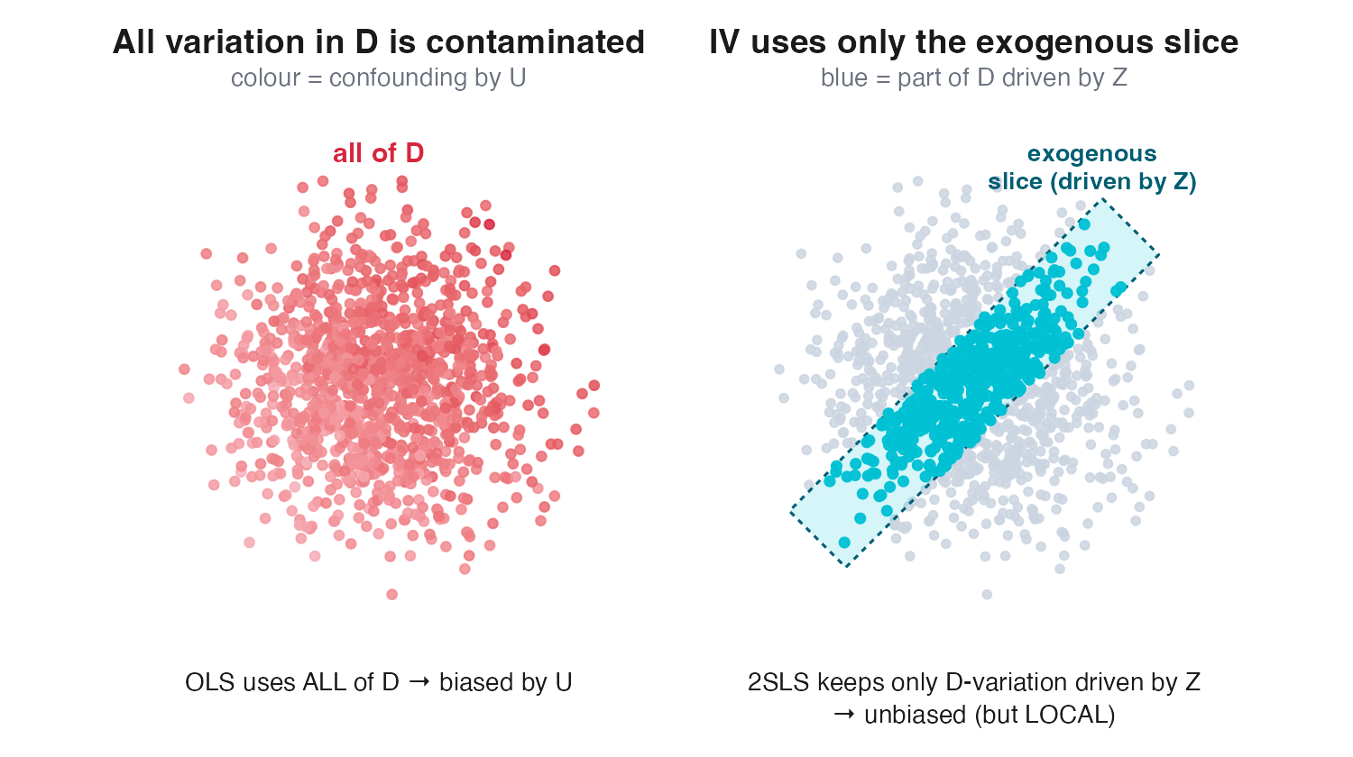
If you cannot block \(U \to D \to Y\), find a slice of variation in D unrelated to U — that exogenous slice identifies τ even when the rest of D is hopelessly confounded.

This is the thesis of the session, so slow down. Picture all the variation in D — most of it is contaminated by motivation U and useless for causal inference. IV does something counterintuitive: it throws almost all of that variation away and keeps only the sliver of D that an external nudge moved. That sliver is, by construction, unrelated to U. We are deliberately discarding variance to buy exogeneity — IV is a variance-DISCARDING device, not a variance-explaining one. That is why IV estimates are noisier than OLS: less data is doing the work, but the data that remains is clean.

Two ways to harvest it: a nudge (IV) or a cutoff (RDD)

IV = a quasi-random nudge Z that shifts D. RDD = a quasi-random cutoff c that flips D. Same intuition, two devices — and both yield LOCAL effects.

These are siblings, not rivals — both manufacture as-good-as-random variation in D, just from different sources. An instrument is a nudge Z that pushes some units toward treatment; a regression discontinuity uses an administrative cutoff c where crossing a threshold flips treatment. I pre-empt over-generalization right here, early, because it’s the single most common student error: both designs recover a LOCAL effect, not the average treatment effect for everyone. IV gives you the effect among those the nudge moved; RDD gives you the effect right at the cutoff. We will name these precisely later — for now, plant the flag that “local” is a feature, not a footnote.

What makes an instrument? The strangeness principle

A valid instrument’s link to the outcome should be puzzling to a smart layperson.

If the only way Z could possibly move Y is through D, then that strangeness is your evidence for the exclusion restriction.

Tech reskin: a randomly-timed reminder banner has no business changing engagement Y — except by getting the user to open the notification (D). Its irrelevance to everything else is the point.

This is the operational recognition test students should carry out of the room. Exclusion is the hardest IV assumption and it’s untestable, so you argue it with a story, not a statistic. The heuristic: explain your instrument to a smart non-economist and watch their face. If they say “why on earth would THAT affect engagement?”, you have a good instrument — the only path from Z to Y runs through D. If they immediately list three other ways Z could matter, exclusion is in trouble. The banner example is deliberately mundane: the timing of a reminder is arbitrary, so it can’t plausibly affect engagement through any channel except prompting the open. Strangeness is a feature.

The encouragement design IS an instrumental-variable design

You can’t withhold a shipped feature from users. But you can randomize a nudge to use it:

• banner / email / pop-up → Z (randomized)
• adoption / opening → D (the user’s choice)
• business metric → Y

This is exactly the FitLife pop-up: randomly shown, it nudges opening without forcing it.

Elbers (2023) document this as Spotify’s industry template for measuring feature effects.

A strong nudge produces a huge first-stage F — foreshadowing the weak-instrument problem.

This is the tech on-ramp, deliberately placed BEFORE any algebra — I want students to see that they have already run instrumental-variable designs without the name. Product teams constantly ship features they cannot ethically or practically withhold, but they CAN randomize who gets encouraged to use it. The randomized encouragement is the instrument Z; whether the user actually adopts is the confounded treatment D; the KPI is Y. Spotify’s engineering blog describes precisely this. End by foreshadowing: in the FitLife lab the pop-up is a strong nudge with a first-stage F around 296 — but we’ll meet a weak variant where F is only about 10.9 and the inference falls apart. That tension drives Act 2.

What the Variation Buys You: Wald, 2SLS, and LATE

A four-step contract: intuition, then identification, then fragility, then field

We will work the same instrument through four questions — in order.

Step	Question	Where
1. Intuition	What is an instrument, and what variation does it buy?	this act
2. What it identifies	Wald, 2SLS — and whose effect is it?	this act
3. When it breaks	Weak instruments, invalid exclusion	Act 2
4. Where tech finds it	Lotteries, nudges, allocation rules, cutoffs	throughout

The discipline: never skip step 2 — an IV that “works” still only answers a question about some people.

This is the Cunningham move (Cunningham 2021): state the teaching contract up front so students always know which question we are on. The act covers steps 1 and 2; weak instruments (step 3) is the next act; field applications are woven throughout. Emphasize the punchline now so it doesn’t surprise them later: even a perfectly valid instrument answers a local question. Transition: start with the picture — three assumptions, one DAG.

Three assumptions, all readable off a single DAG

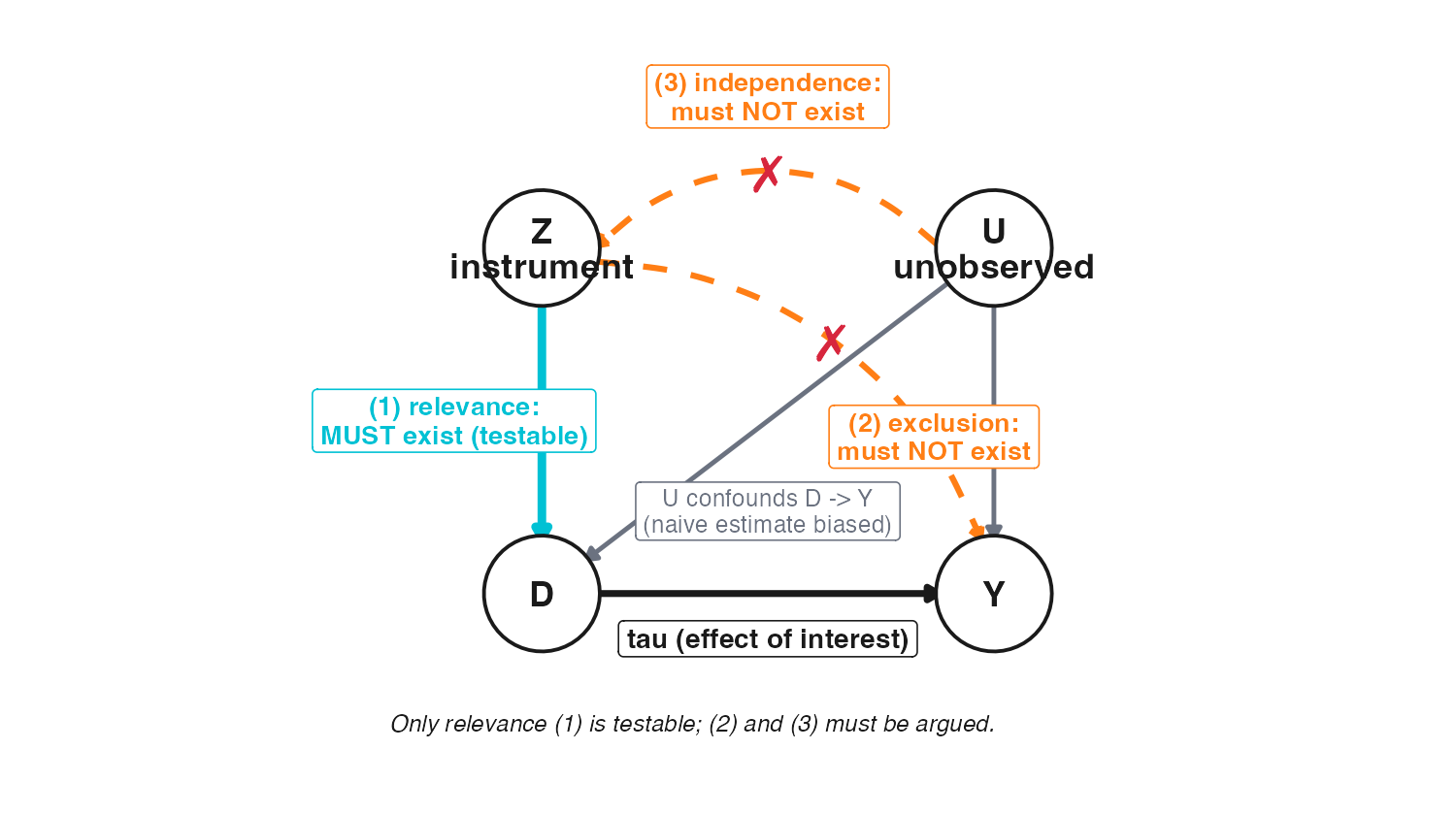
What each arrow must (not) be

(1) Relevance — Z → D MUST exist (and is testable).   (2) Exclusion — a direct Z → Y must NOT exist.   (3) Independence — U → Z must NOT exist.   SUTVA underlies all three.

Walk the DAG node by node. The whole IV idea: U confounds D → Y, so the naive D-on-Y comparison is biased; we import clean variation from Z. For Z to launder that bias it must move D (relevance), affect Y only through D (exclusion), and itself be unconfounded by U (independence). The framework is Imbens and Angrist (1994) and Angrist, Imbens, and Rubin (1996). SUTVA — no interference, one version of treatment — sits beneath everything, exactly as in the potential-outcomes setup from S05. Transition: notice only one of these three arrows is something the data can confirm.

Finally — a testable assumption (and only one of three)

Relevance — checkable

The first stage Z → D shows up in the data. Run the regression, read the coefficient, read the F-statistic. If Z does not move D, you find out.

Exclusion + independence — argued

No regression certifies these. You defend them from institutional knowledge: how the instrument was assigned, and what else it could plausibly touch.

Most of the discipline lives in the argument, not the F-statistic. A strong first stage does not make an instrument valid.

This is the slide students must internalize. After two sessions of “you can never test no-unobserved-confounding,” relevance is a relief — it is genuinely testable. But that relief is dangerous: it tempts people to treat a big F as a validity certificate. Exclusion and independence are defended with words and institutional detail, never with a p-value. The lottery is independent because a computer drew numbers; the encouragement banner is excludable because we can argue it changes only whether you open the app. Transition: let’s drill the argument muscle.

Valid or invalid? Four instruments, four verdicts

Proposed Z → D → Y	Verdict
(a) Firm size → R&D spend → patents	INVALID — size affects innovation directly (exclusion fails)
(b) Distance to training center → training → productivity	VALID — distance plausibly touches productivity only via training
(c) A new budget-allocation rule → ad spend → sales	VALID — rule-driven variation is as-good-as-random across units
(d) Firm profitability → benefits → satisfaction	INVALID — profitability drives satisfaction directly

A live tech threat

The Spotify encouragement banner (Elbers 2023) might itself lift engagement — seeing the banner nudges you even if you never click. That is a direct Z → Y path: an exclusion violation. In FitLife the reminder’s wording is the design lever: a bare trigger (“1 new notification”) is far more excludable than a motivational banner (“Keep your streak alive!”) that can lift engagement with no open.

Run this as cold-call. Read each row, pause, ask the room “valid or invalid — and which assumption?”, then reveal. (a) and (d) fail exclusion the same way: the “instrument” is really a confounder with its own arrow into Y. (b) and (c) work because the variation has a clean as-good-as-random source — geography, or an administrative rule that no individual unit chose. The Spotify case is the subtle one and the most relevant to your students: a banner designed as encouragement can have a direct psychological effect on engagement, breaking exclusion. That is why encouragement designs report the threat explicitly. Transition: granting validity, what number does IV actually compute?

The Wald estimand: the nudge’s effect on Y, scaled by how much it moved D

With a binary instrument — and, for now, one effect \(\tau\) shared by everyone:

\[\tau \;=\; \frac{E[Y\mid Z=1]-E[Y\mid Z=0]}{E[D\mid Z=1]-E[D\mid Z=0]} \;=\; \frac{\text{reduced form}}{\text{first stage}}\]

Numerator — reduced form. How much the nudge moves the outcome: the effect of \(Z\) on \(Y\).

Denominator — first stage. How much the nudge moves take-up: the effect of \(Z\) on \(D\).

The nudge shifts \(D\) by the first stage; with a constant effect that shift carries through to \(Y\) at rate \(\tau\), so reduced form \(= \tau \times\) first stage — rise over run.

If a banner shifts opens by 16 points and lifts minutes by 1.3, the effect of opening is \(1.3 / 0.16 \approx 8\).

The conceptual heart of IV in one line — kept deliberately in the constant-effect world. The numerator is the reduced form, the effect of the nudge on the outcome (\(Z \to Y\)); the denominator is the first stage, the effect of the nudge on take-up (\(Z \to D\)). The logic is rise-over-run: the instrument shifts \(D\) by the first-stage amount, and because — for now — a single \(\tau\) links \(D\) to \(Y\), that shift propagates to \(Y\) as reduced form \(= \tau \times\) first stage, so \(\tau\) = reduced form / first stage. Use the FitLife numbers live: the encouragement moves opens by about 16 points and lifts engagement by about 1.16, recovering roughly 8 — the true effect — versus the biased OLS of 11.3. Deliberately hold the ITT / complier-share reading until we drop homogeneity a few slides on; here there is one effect and one number. Transition: same object falls out of a covariance formula too.

The same object, the covariance view: Cov(Y,Z) over Cov(D,Z)

For a general (not just binary) instrument, the identical estimand is:

\[\tau \;=\; \frac{\operatorname{Cov}(Y,Z)}{\operatorname{Cov}(D,Z)}\]

Difference-in-means view (binary Z): the Wald ratio of two contrasts.

Covariance / regression view (any Z): how Z co-moves with Y, scaled by how Z co-moves with D.

Two angles, one estimand. The covariance form is what generalizes to 2SLS with continuous instruments and controls.

Reassure students this is not a new method — it is the same Wald object written for a continuous instrument. With binary Z, Cov(Y,Z)/Cov(D,Z) algebraically collapses to the difference-in-means ratio on the previous slide; verify that informally if the room is comfortable with covariance algebra. The point of showing both is that the covariance/regression view is the bridge to 2SLS: once Z or D is continuous, or once we add controls, the ratio-of-differences picture stops working but the covariance picture keeps going. Transition: 2SLS is exactly this, with controls — and it has a clean DAG interpretation.

2SLS is the Wald ratio with controls — and it is DAG surgery

Stage 1 project D on Z (and X) → predicted \(\hat{D}\).   Stage 2 regress Y on \(\hat{D}\). Replacing D with \(\hat{D}\) severs U → D — U no longer touches the purged treatment.

Linear constant-effects model: \(Y = \tau D + X\beta + \varepsilon\), one constant slope \(\tau\). Linearity is a real assumption for continuous \(D\); for binary \(D\) (FitLife) it is automatic.

Give them the surgery intuition: D is contaminated because U flows into it. Stage 1 keeps only the part of D explained by the clean instrument (and controls), discarding everything correlated with U. That predicted D-hat is, by construction, orthogonal to U — so when we regress Y on D-hat, the U → D arrow has been cut and the back-door is closed. This is why we draw it as graph surgery, paralleling the do-operator surgery from S02. One firm caveat to plant now: this clean story assumes a constant effect. Under heterogeneity, what 2SLS recovers is a LATE, not the ATE — we will earn that distinction over the next few slides. Do not oversell. Transition: a practical warning before the conceptual pivot.

Never run 2SLS by hand — the second stage gets the standard errors wrong

By hand (two separate regressions): the point estimate is right, but the SEs are wrong — stage 2 treats \(\hat{D}\) as if it were observed data, ignoring that it was estimated.

Use a real IV routine: it propagates first-stage uncertainty correctly. Cluster SEs at the assignment level.

feols(Y ~ X | D ~ Z)   # fixest: controls X, instrument Z for D

R: ivreg / fixest::feols.   Python: linearmodels.IV2SLS. The lab uses these; hand-rolled 2SLS is a common, silent bug.

Cheap, high-value practical point. Students who learned the two-stage recipe literally will sometimes run two lm()/lm() calls — the coefficient matches, so they trust it, but the reported SEs are too small because stage 2 does not know D-hat carried estimation noise. A canned IV estimator gets the variance right. Stress clustering at the level of randomization — in FitLife, the assignment level — exactly as in the A/B testing inference discussion. The one code line is all they need to recall; the lab walks the full call. Transition: now the conceptual pivot the whole act has been building toward.

Drop homogeneity: IV identifies a local effect, not the global ATE

So far Wald / 2SLS read as the global ATE — which holds as long as either homogeneity does:

Same effect

One constant \(\tau\) — everyone responds to \(D\) alike.

Same compliance

Z moves every unit’s \(D\) — full compliance.

Reality breaks both: effects vary, and Z moves only some units’ \(D\) — not all.

The consequence

The instrument speaks only for the units it moves ⇒ IV gives a local ATE (the movers’ average), and only under monotonicity (no defiers). (Imbens and Angrist 1994)

→ which units move, which don’t? The four compliance types.

The hinge of the act — the move from ATE to LATE, the 2021-Nobel contribution of Angrist and Imbens. Make the logic explicit: the global-ATE reading survived if either homogeneity held — one common effect (so the average over movers equals the average over all), OR full compliance (so the instrument moves everyone and there is no “rest” left for it to be silent about). Reality breaks both at once: effects vary — especially in tech, where a feature helps some and does nothing for others — and a nudge moves only a subset. The instant both fail, an instrument observes only the units whose D it changes and is silent about the others, so no valid-instrument machinery returns the ATE — genuine non-identification, not a small-sample nuisance. The fix is a behavioral restriction, monotonicity, which buys the local effect among compliers. Transition: to see who the movers are, catalogue the four compliance types.

Four compliance types — only compliers are visible to the instrument

Defined by \((D(Z{=}1),\,D(Z{=}0))\): always-takers (1,1), never-takers (0,0), defiers (0,1), compliers (1,0). Always- and never-takers ignore Z entirely.

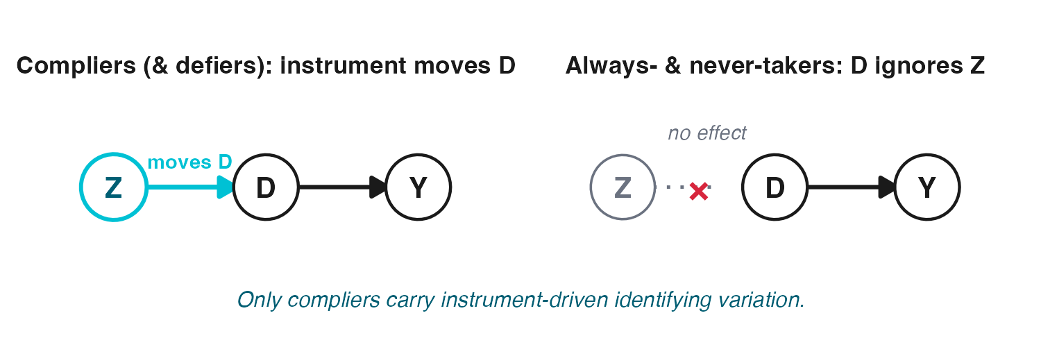
But the stratum is latent — each observed \((Z,D)\) cell fits two types:

	D = 0  (didn’t take)	D = 1  (took)
Z = 0	never-taker or complier	always-taker or defier
Z = 1	never-taker or defier	always-taker or complier

Make this first-person with the Vietnam draft (Angrist 1990). “I’d serve whether or not my number came up” — always-taker. “I’d dodge no matter what” — never-taker. “I serve only because I was drafted” — complier. “I serve only because I was NOT drafted, and would have dodged if drafted” — defier, the perverse type. The key visual point in the figure: only compliers (and defiers) have an arrow from Z to D; always- and never-takers’ treatment is fixed regardless of the instrument, so they contribute zero identifying variation. The instrument is blind to their treatment effect. Transition: assume defiers away and the algebra simplifies beautifully.

Monotonicity kills the defiers — and the math leaves only compliers

Assumption — Monotonicity (no defiers)

\(\forall i:\ \ D_i(Z{=}1) \ge D_i(Z{=}0)\) — the instrument moves everyone weakly the same direction.

Under exclusion, always- and never-takers contribute 0 to the reduced form — Z doesn’t change their D, so it can’t change their Y.

With defiers assumed away, only compliers move with Z — so the Wald ratio is exactly their average effect.

What survives in both numerator and denominator is compliers only — the local average treatment effect (LATE). The estimator is unchanged; only whose effect it is has been pinned down.

This is the derivation in words. Exclusion zeroes out the always/never-takers in the numerator: the instrument literally does not alter their treatment, so by exclusion it cannot alter their outcome — they wash out of the reduced form. Monotonicity removes the defiers, who would otherwise enter with the opposite sign and contaminate the average. What remains in both numerator and denominator is compliers only, so the Wald ratio is exactly the average treatment effect among compliers. Stress that monotonicity is a behavioral assumption — defensible for a nudge (nobody is less likely to open because they were encouraged) — and like exclusion it is argued, not tested. Transition: name the object and the price we paid.

So the Wald ratio identifies a LATE — compliers, not everyone

Local Average Treatment Effect (LATE / CACE)

\(\text{LATE} \;=\; \mathbb{E}\big[\,Y_i(1) - Y_i(0) \,\mid\, \text{complier}\,\big]\)  —  the effect for the only stratum the instrument moves.

Identification (binary Z, D; independence, exclusion, monotonicity)

\(\dfrac{\mathbb{E}[Y\mid Z{=}1]-\mathbb{E}[Y\mid Z{=}0]}{\mathbb{E}[D\mid Z{=}1]-\mathbb{E}[D\mid Z{=}0]} \;=\; \dfrac{\text{ITT}}{\text{complier share}} \;=\; \text{LATE}\)

If compliers are ~16% of users, the LATE describes that 16% — not always-takers, not never-takers.

The punchline of the act. IV does not buy you the ATE for free; it buys you a clean estimate of a local effect, and the locality is the price of the instrument. Read the five assumptions a LATE rests on — SUTVA · Independence · Exclusion · Relevance · Monotonicity — as a checklist students should run through for any IV they encounter or build (monotonicity is the one we just added; the other four carried over from the identification slides). Make the complier-share concrete with FitLife: about 16% complier share, so the LATE is the per-opener effect for that 16% who open only because they were encouraged — a precise, valid, but local number. We return to treatment-effect heterogeneity in S09. Transition: so which number does a manager actually want?

ITT and LATE answer different business questions

	Business question	What it tells you
ITT	“Should we ship the nudge to everyone?”	the rollout number — effect of the policy as deployed
LATE	“What does adoption do for those it moves?”	the product-understanding number — effect of the behavior

The tempting wrong answer

Computing the ATE with respect to \(D\) compares adopters to non-adopters directly. This comparison is biased by self-selection, as they differ in \(U\).

Land the act on the decision, not the estimator. ITT and LATE are both legitimate — they answer different managerial questions, and choosing wrong is a real error. If you are deciding whether to roll a banner out to the whole base, the ITT (effect of offering, averaged over compliers and the unmoved) is the relevant number. If you are trying to understand what the feature itself does to a user who takes it up, the LATE is what you want. The naive move — compare people who adopted to people who didn’t — looks like it answers the second question but is contaminated by self-selection on U, which is exactly the OLS-11.3-versus-truth-8 gap from the FitLife lab. Foreshadow Assignment III: students will reconcile the effect of SENDING (about +7.6 min, part direct, part by inducing opens) against the LATE of OPENING (about +8 min among compliers) — and must not collapse them into a single clean number. Framework reference: Angrist and Pischke (2009) and Angrist and Pischke (2015).

When the Variation Is Too Thin: Weak Instruments

A weak instrument is a nudge that barely moves D

If \(Z\) barely moves \(D\), almost no one is a complier and the LATE denominator collapses — so strength is the one IV property you measure, the first-stage F:

\[D = \pi_0 + \pi_1 Z + \mathbf{X}'\boldsymbol\gamma + v, \qquad H_0:\ \pi_1 = 0\]

\[F \;=\; \underbrace{\frac{\big(\mathrm{RSS}_{D\sim\mathbf{X}} - \mathrm{RSS}_{D\sim Z,\mathbf{X}}\big)/q}{\mathrm{RSS}_{D\sim Z,\mathbf{X}}/(n-k)}}_{\text{gain in fit}} \;=\; \underbrace{\frac{\hat\pi'(Z'Z)\,\hat\pi}{q\,\hat\sigma_v^2}}_{\text{signal / noise}} \qquad {\small q=\#\text{ excl. instruments}}\]

• Two readings, one number: the RSS drop from adding \(Z\) equals \(\hat\pi'(Z'Z)\hat\pi\), so “gain in fit” = “signal / noise” — and by FWL both partial out \(\mathbf{X}\).
• Covariates partialled out, not tested — only the excluded instrument(s) enter. Report this partial F (Cragg–Donald / Kleibergen–Paap), not the overall regression F.
• \(q=1\): \(F = t^2 = \big(\hat\pi_1/\mathrm{SE}(\hat\pi_1)\big)^2\), the squared t of the \(D\)-on-\(Z\) coefficient — weak = imprecise, not small.

The conceptual hinge of the act, and the one IV property you can actually measure. The first stage is the denominator of the Wald/LATE ratio; the first-stage F tests the null that the excluded instrument’s coefficient is zero, H0: pi1 = 0. Formalize the role of covariates: X enters BOTH the restricted model (D on X) and the unrestricted model (D on Z and X); the F is the gain in fit from adding the instrument(s), scaled by residual variance and the number of excluded instruments q. By Frisch-Waugh-Lovell this equals the F of the X-residualized D on the X-residualized Z, so the covariates are partialled out, never part of the null. Two practical consequences: (1) report the PARTIAL first-stage F — Cragg-Donald under homoskedasticity, Kleibergen-Paap with robust/clustered errors — NOT the overall regression F, which strong controls would inflate and which would hide a weak instrument; (2) just-identified (q=1) it is exactly the squared t on the single D-on-Z coefficient, F = t^2, so “weak” means imprecise, not small in magnitude. The rest of the act: how big F must be (rule of thumb 10, Lee 104.7), the effective F under clustering, and weak-IV-robust inference. Students estimate these first-stage F’s on the lab data.

Two dangers: the cure becomes the disease, and the precision is fake

Danger 1 — bias. As the first stage weakens, 2SLS is pulled toward the biased OLS plim; relative bias \(\approx \tfrac{1}{F+1}\), so at \(F\to 0\) the IV is no better than OLS (Bound, Jaeger, and Baker 1995).

Danger 2 — false precision. The reported CI looks tight, but it under-covers: the true coverage of a “95%” interval is far below 95%.

Two failure modes, and students conflate them. Danger 1 is bias: the curve shows relative bias of 2SLS-to-OLS as a function of the first-stage F, well approximated by 1/(F+1). At F near zero the bias is 100% of the OLS bias — the instrument has bought you nothing, and worse, weak instruments amplify even a small violation of exclusion (the small bias in the numerator gets divided by a small first stage). This is Bound, Jaeger and Baker’s classic warning. Danger 2 is subtler and more dangerous in practice: false precision. The conventional 2SLS standard error is derived under strong-instrument asymptotics; when the instrument is weak, the sampling distribution is non-normal and fat-tailed, so the nominal 95% interval covers the truth far less than 95% of the time. The vertical markers (F=10 rule of thumb, F=104.7 honest-5% threshold) foreshadow the next four slides.

See it: the estimate degrades as the first stage weakens

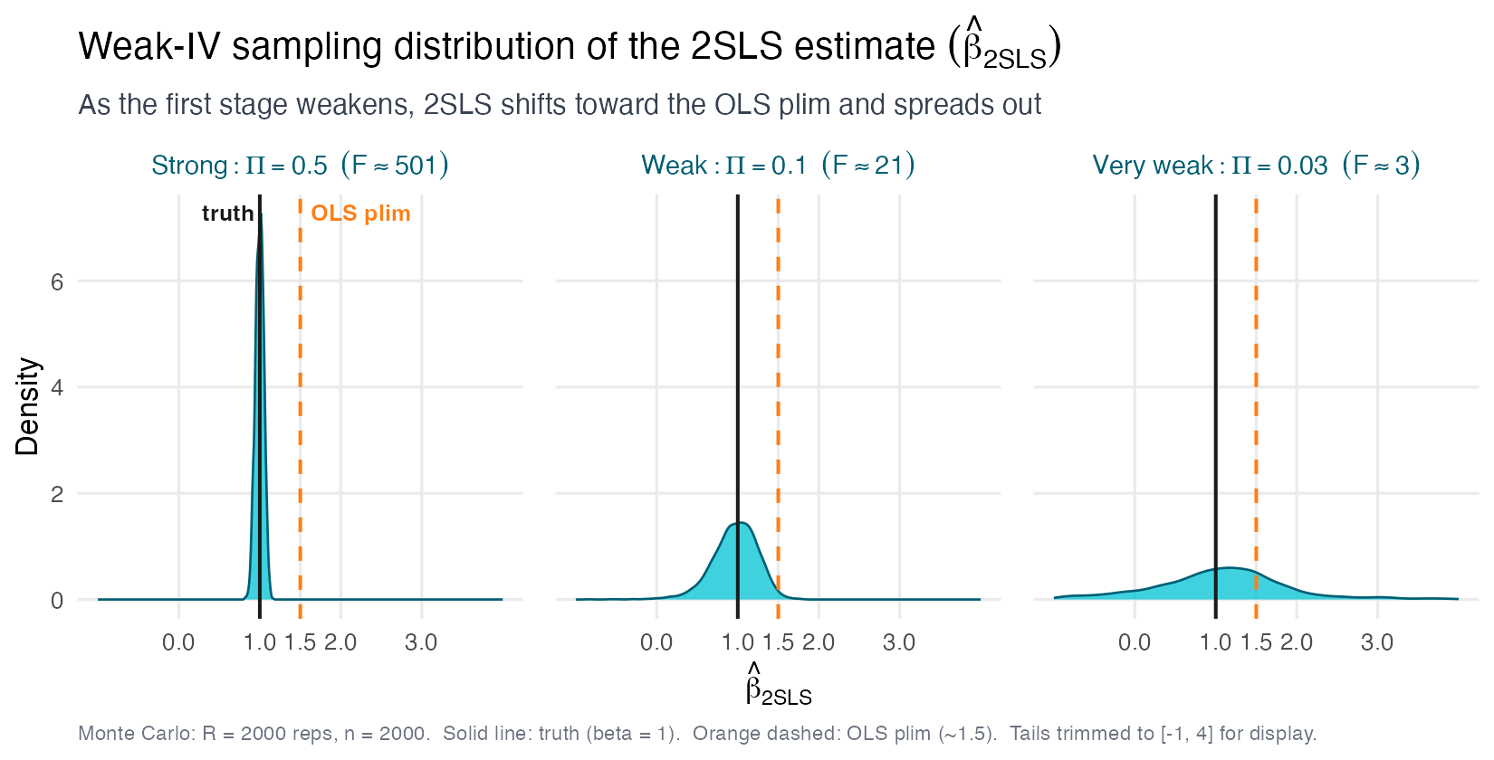
Simulated DGP: \(Y = \varepsilon,\ D = \Pi\, Z + \eta\) with \(\mathrm{corr}(\varepsilon,\eta)>0\). Step \(\Pi\) down and the 2SLS distribution drifts off the truth toward the OLS plim and fattens.

This is the bias curve made tangible — and it previews the lab demo students run next session. The data-generating process is deliberately stark: the true effect of D on Y is set so the solid black line is the truth, while confounded OLS would land on the orange dashed plim. Three panels step the first-stage strength Pi down from 0.5 (F about 501) to 0.1 (F about 21) to 0.03 (F about 3). In the strong panel the 2SLS distribution is a tight spike right on the truth. As Pi shrinks, two things happen at once — exactly the two dangers from the previous slide: the center drifts away from the truth toward the OLS plim (bias), and the distribution fattens into long tails (false precision, because a single reported SE cannot describe that spread). Tell them: the lab reproduces this in a few lines of R/Python, and they will watch their own estimate degrade as they dial Pi down.

“F > 10” is a screen, not a certificate

The famous rule of thumb: a first-stage \(F > 10\) flags an instrument as “not catastrophically weak” (Staiger and Stock 1997). Stock and Yogo (2005) made it precise — tabulated critical values for a chosen bias or size tolerance.

What the threshold quietly assumes

• It bounds only the tolerance you picked (e.g. “2SLS bias under 10% of OLS bias”) — not a clean pass/fail for your estimate.
• It is derived under homoskedasticity and a single instrument.
• It is a floor, not a finish line: bigger is genuinely better — the bias curve keeps falling well past 10.

Decouple the ritual from the logic. Staiger and Stock proposed F>10 as a quick screen; Stock and Yogo turned it into a proper table of critical values, but each row answers a specific question — “what F do I need so that 2SLS bias is at most 10% of OLS bias?” or “so that the true size of a nominal 5% test is at most 15%?” The number 10 corresponds to one such tolerance, not to truth. Three caveats students must internalize: (1) it certifies a tolerance you implicitly chose, not your particular estimate; (2) it assumes homoskedastic, non-clustered errors and is cleanest with one instrument; (3) it is a minimum bar — reading the bias curve, going from F=10 to F=40 still meaningfully cuts bias, so do not treat 10.1 as “safe and done”. This sets up the next two slides: under real data the naive F is the wrong number, and even a correct F>10 is too lenient.

With real (heteroskedastic, clustered) data, report the EFFECTIVE F

The classical F (previous slide) needs i.i.d. errors; clustered data needs a robust version — three names, one job:

First-stage statistic	What it is
Cragg–Donald F	the classical F (one treatment) — homoskedastic
Kleibergen–Paap rk Wald F (Kleibergen and Paap 2006)	its cluster-robust version (robust Cragg–Donald) — what ivreg2 / ivreghdfe print
Effective F (Montiel Olea and Pflueger 2013)	a different robust statistic with valid critical values — compare to its own (Montiel Olea–Pflueger) threshold, not 10

What to use: i.i.d. → classical F vs \(10\); clustered → the effective F vs its critical value. One instrument: all three are the same number — read the robust first-stage F (Python linearmodels, R fixest / ivreg). Several: the dedicated effective F via ivDiag (R).

This is the slide that makes the rule of thumb usable on the data students will actually analyze. The classical first-stage F is built on homoskedastic, independent errors. Encouragement experiments at Spotify or Facebook violate both: variance depends on covariates, and observations cluster by user, geography, or week. Andrews, Stock and Sun (2019) recommend judging strength by the effective F of Montiel Olea and Pflueger, compared to ITS OWN critical value (not the homoskedastic 10). The catch students must hear: the Kleibergen-Paap rk Wald F that ivreg2 / ivreghdfe print is the robust Cragg-Donald — NOT automatically the effective F. But with a single instrument the classical, KP rk, and effective F all collapse to the squared robust t, so in a one-instrument encouragement design you just read off the robust first-stage F your software prints. With SEVERAL instruments they diverge, so use a dedicated effective-F routine — R ivDiag::eff_F. Python has no turnkey effective-F: for one instrument linearmodels’ robust first-stage F is the same number, and for robustness you fall back on Anderson-Rubin inference (the ivmodels package). Punchline: the threshold logic survives, but feed it the robust statistic. Next slide raises the bar on the threshold itself.

F > 10 is too lenient for honest 5% inference

Lee et al. (2022) ask a sharper question: what first stage do you need so that a nominal 5% t-test on the 2SLS estimate truly rejects at 5%?

The honest threshold is much higher

A nominal 5% t-test has 5% size only if the first-stage F > 104.7 — not 10.

The tF procedure swaps the fixed \(1.96\) for a critical value \(\hat c(\hat F)\) indexed by the observed first stage, so the 95% CI becomes

\[\hat\beta \;\pm\; \hat c(\hat F)\cdot \widehat{\mathrm{SE}}(\hat\beta), \qquad \hat c(\hat F)\ge 1.96,\quad \hat c = 1.96 \iff \hat F \ge 104.7.\]

\(\hat c(\hat F)\) shrinks smoothly to \(1.96\) as \(\hat F\) grows — a weaker first stage automatically widens the interval, with no cliff-edge pass/fail.

This is the slide that should unsettle them. Lee, McCrary, Moreira and Porter reframe the question around the inference we actually report: not “how biased is 2SLS?” but “if I run the standard t-test at the 5% level, does it actually have 5% size?” The answer is that you need a first-stage F above 104.7 for the conventional t-test to be honest — an order of magnitude beyond the folk rule of 10. Rather than a new cliff, they offer the tF procedure: a smooth standard-error inflation factor indexed by the observed F, so weaker first stages automatically get wider, honest intervals. Then drive it home with the lab’s weak variant: F is about 10.9, so it sails past the F>10 ritual, yet the 2SLS interval still includes zero — the screen gave a false all-clear. That failure motivates the safety net on the next slide.

The safety net: weak-IV-robust inference (Anderson–Rubin)

When you cannot trust the F, stop relying on the 2SLS standard error and switch to an interval that is valid regardless of instrument strength.

Anderson–Rubin confidence sets

Invert a test on the reduced form: for each candidate \(\beta_0\), regress \(Y-\beta_0 D\) on \(Z\) (and controls \(\mathbf{X}\)) and test \(H_0\): coefficient(s) on \(Z\) \(=0\). Keep every \(\beta_0\) the data do not reject — \[\text{AR set} = \big\{\beta_0 : \mathrm{AR}(\beta_0)\le F^{\alpha}_{k,\,n-k-p}\big\},\quad \mathrm{AR}(\beta_0)=\frac{(Y-\beta_0 D)'P_{\tilde Z}(Y-\beta_0 D)/k}{(Y-\beta_0 D)'M(Y-\beta_0 D)/(n-k-p)}.\] No first stage in the denominator → correct coverage at any strength; just-identified (\(k=1\)) it is the most powerful weak-robust test (Anderson and Rubin 1949).

When the instrument is weak the AR set comes out wider than the under-covering 2SLS t-interval — that width is the honest signal. Andrews, Stock, and Sun (2019): report the effective F; if it is borderline or just-identified, report AR sets.

Here is the constructive payoff. The Anderson-Rubin approach inverts a test that does not require the first stage to be strong — it builds the confidence set from the reduced-form fit directly, so its coverage is correct whether F is 300 or 0.3. In the just-identified case (the typical encouragement design: one instrument, one treatment), AR is also the most powerful weak-robust test, so you lose nothing by using it. Connect to the previous slide: when the instrument is weak the AR interval comes out wider than the 2SLS t-interval — and that is the point, the t-interval was too narrow and under-covering, while AR honestly reflects how little the thin instrument identifies. Andrews, Stock and Sun give the field-standard recipe students should memorize: always report the effective F, and when it is borderline or the design is just-identified, report AR sets alongside (or instead of) the t-interval. That recipe is the checklist on the next slide.

Weak-IV checklist to take to the lab

Five rules for any IV estimate you report

1. Always report the first-stage F — the effective / Kleibergen–Paap version under heteroskedasticity or clustering, never the naive homoskedastic one.
2. Bigger than 10 is genuinely better. Treat 10 as a floor, not a finish line; honest 5% inference wants far more.
3. When in doubt or just-identified, use Anderson–Rubin CIs — correct coverage at any strength.
4. Report the ITT alongside the IV estimate. The reduced-form effect needs no first stage and anchors what the data actually show.
5. A noisy weak-IV estimate can be worse than careful OLS — IV is not automatically the safer choice.

The take-home card. Walk each line once. (1) The F is non-negotiable and must be the robust one — tie back to Montiel Olea-Pflueger and Kleibergen-Paap. (2) Reframe 10 as a floor; the bias curve and Lee et al.’s 104.7 both say more is better. (3) AR is the default safety net for borderline or just-identified designs. (4) Reporting the intention-to-treat / reduced-form effect is the underrated discipline — it requires no first stage, cannot be inflated by a weak denominator, and in the assignment students will see the effect of sending the email (about +7.6 minutes) sit honestly beside the LATE of opening it (about +8 minutes among compliers). (5) The cultural correction: a confounded but precise OLS estimate can beat a “clean” IV estimate that is too noisy to learn anything from — IV earns its keep only when the instrument is strong and the exclusion logic holds. This checklist is exactly what they execute in the lab and in Assignment III. Transition: now that we can diagnose strength, the next act surveys the design family that supplies real-world instruments.

Where Tech Harvests Variation: the IV Design Family

Where do good instruments come from? Two sources

A valid Z must be as-good-as-randomly assigned and affect Y only through D. Two families deliver this:

1. Lotteries — purely random

• Encouragement / nudge experiments
• Draft, admission, prize lotteries
• Oversubscribed-program lotteries

Randomness you run.

2. Natural experiments — as-good-as-random

• Policy & regulation shocks
• Decision-maker variation
• Economic shocks, geography, weather

Randomness you find.

The art of applied IV is recognizing where the world has already done the randomizing for you (Angrist and Krueger 2001).

Frame the whole act: we have the machinery (2SLS, LATE, weak-IV diagnostics) — now where do real instruments come from? Two buckets. The first you literally run as an experiment; the second you discover in administrative or market data. Angrist and Krueger’s “Instruments for Causal Inference” survey is the canonical catalogue. The rest of the act walks bucket-by-bucket through the families tech firms actually use, then hands off to RDD as a special sixth case.

Lotteries: the gold-standard instrument by construction

A lottery randomizes eligibility, not treatment — which makes the assumptions credible by design.

Why the assumptions hold

• Independence: the draw is random, so \(Z \perp U\) — guaranteed, not assumed.
• Exclusion: winning a lottery has no path to Y except through the program.

The catch: imperfect take-up

Winners don’t all comply; losers sometimes get in anyway. Z shifts the probability of D, not D itself.

\[\tau_{LATE} = \frac{\text{ITT}}{\text{take-up}}\]

Scaling ITT by the take-up rate converts a “lottery-win” effect into the effect of actually receiving treatment, for compliers.

This is the conceptual anchor of the lecture: lotteries make independence and exclusion true by construction rather than by argument. Stress that randomizing eligibility is not the same as randomizing treatment — almost no lottery achieves 100% take-up, which is precisely why we need IV/LATE rather than a simple comparison of means. The ITT-over-take-up formula is the Wald estimator from Act 1, now read as “rescale the reduced form by the first stage.” Connect to FitLife: the encouragement was the lottery, opening the email was the take-up.

Tech lotteries: oversubscribed betas, waitlists, and the patent “lottery”

Capacity constraints — and the A/B tests you already run — turn ordinary product decisions into clean lotteries.

Setting	Instrument Z	Treatment D	Outcome Y
Oversubscribed beta / waitlist	Random invite	Uses feature	Retention, revenue
Public-health program	Lottery win (Finkelstein et al. 2012)	Enrolls in coverage	Utilization, health
School admission	Seat lottery (Abdulkadiroğlu et al. 2011)	Attends school	Test scores
Patent grant	Examiner assignment (Farre-Mensa, Hegde, and Ljungqvist 2020)	Patent granted	Firm growth
Online ad A/B test	Random ad assignment (Gordon et al. 2019)	Actually sees the ad	Conversion, sales

Winning raises P(use D) but not to 100% — the Oregon / charter-lottery structure.

The point: a capacity-constrained beta invite is not “a marketing tactic” — it is the Oregon Medicaid lottery wearing a hoodie. Finkelstein et al. used Oregon’s 2008 Medicaid lottery; Abdulkadiroglu et al. used Boston/NYC charter seat lotteries. Both have exactly the imperfect-take-up structure of last slide. The patent case is subtler: it is a quasi-lottery — examiners are conditionally randomly assigned, and lenient examiners grant more patents — which is also a leniency design (we return to it in S40). Tell students: if you ever ration access randomly, archive the randomization; it is a free instrument. The ad A/B-test row is the same machinery from the other direction — random assignment instruments actual exposure (many assigned users skip or ad-block), so 2SLS turns ITT into the per-exposure effect (LATE = ITT / take-up). Gordon et al. (2019) showed observational ad measurement is badly biased against this experimental benchmark at Facebook.

Natural experiments: randomness you find

When you cannot run an experiment, find an event that is as-good-as-random — then pin down what it instruments.

Randomness you find — Z → D → Y	↳ But what else moved with Z?
Privacy rollout. iOS-14.5 timing (Z) → cross-app tracking on/off (D) → ad revenue/user (Y)	it also changed attribution & performance
Surge pricing. A hyper-local rain shock (Z) → surge multiplier shown (D) → booking conversion (Y)	rain also lifts ride demand directly
Latency. A CDN-edge incident (Z) → page-load delay felt (D) → checkout conversion (Y)	a wider outage also hits payment gateways & rivals
Recommender noise. Ranker perturbs what’s surfaced (Z) → item exposure (D) → click-through (Y) (Sharma, Hofman, and Watts 2015)	a new slot shifts attention, not just exposure

The honest caveat

Each arrow is a claim, not a fact — and usually only conditional on X.

So ask what else moved with Z? You must argue and balance-test the randomness — never just assert it, or exclusion fails.

The credibility hinge of the whole observational-IV enterprise: a natural experiment is a claim, not a fact — the burden is on you to show that whatever generated Z is unrelated to U. Walk the four table rows; each is as-good-as-random only conditional on X, and the right column is its live exclusion threat:

• Privacy rollout (Apple ATT, iOS 14.5, Apr 2021): upgrade timing strips the cross-app IDFA tracking signal D, which moves ad revenue Y. Threat: iOS 14.5 bundled SKAdNetwork attribution + performance changes on the same date, and privacy-eager users upgrade earlier — so timing can hit Y off the tracking channel. (GDPR’s 25-May-2018 EU enforcement deadline is the regulatory cousin.)
• Surge pricing (rain → surge multiplier → rider conversion): rain tightens supply vs. demand, so the algorithm raises the price D. Threat: rain is a two-sided shock — it also lifts ride demand and willingness-to-pay directly, so Z reaches Y off-price. Defensible only with zone × hour × weekday × season fixed effects.
• Latency (CDN-edge incident → page-load delay → checkout): a degraded route slows the page D. Threat: a wider regional outage also takes down payment gateways and rivals, so scope Z to a single-provider, single-site incident and balance-test pre-outage covariates.
• Recommender noise (random ranking jitter → item exposure → click-through): here the recsys itself emits the randomness — the platform-native natural experiment, and the one genuine fitted IV of the four. Sharma, Hofman, and Watts (2015) (Microsoft) used recommender-induced traffic as an instrument to separate causal browsing from baseline demand. Threat: a perturbed slot changes attention/position, not only exposure, and the exploration must be genuinely random, not quality-chasing.

The discipline that separates a design from a story: balance pre-treatment covariates across Z, look for pre-trends, pre-register the exclusion argument. One honesty note for advanced students — the world/policy chains (ATT, GDPR) are usually run as difference-in-differences / reduced-form, not a fitted 2SLS; the IV/LATE reading is the clean teaching frame, whereas the recommender jitter is a genuine fitted IV. Next: a reusable template for finding routing randomness — judge/examiner leniency.

Judge/examiner leniency: a reusable recipe

A surprisingly general template appears wherever cases are routed to decision-makers.

The three-ingredient recipe

1. A pipeline. Units flow through a process to a single decision point (grant / deny, approve / reject, flag / clear).
2. Random routing. Decision-makers are (as-good-as) randomly assigned to cases — conditional on the office × time cell.
3. Differing leniency. Decision-makers differ in how often they treat.

Then the assigned decision-maker’s leniency instruments the treatment: lenient-judge cases are more likely to be treated, but the judge touches Y only through that one decision.

Walk the three ingredients slowly — students will reuse this in the lab and the assignment. The classic is criminal sentencing (random judge assignment), but the structure is everywhere: bail judges, disability examiners, asylum officers, loan officers, patent examiners, content moderators. The instrument is not “the judge” but “how lenient the assigned judge is,” measured from their other cases. Ingredient 2 is what buys independence; ingredient 3 is what buys a first stage. The next two slides fix how to measure leniency and what can go wrong.

Construct leniency the right way: leave-one-out, demeaned within the cell

The instrument is the decision-maker’s treatment rate — but built carefully to avoid mechanical bias.

Two fixes, both essential

• Leave-one-out (jackknife): compute the judge’s treatment rate on all their other cases, excluding case \(i\).
• Demean within the cell: subtract the office × time-period mean.

\[Z_i = \bar{D}_{-i,\,j(i)} - \bar{D}_{\text{cell}(i)}\]

Leave-one-out breaks the mechanical link to \(i\)’s own outcome.

Demeaning ensures Z varies only within the cell where assignment is random.

Without leave-one-out, case \(i\)’s own decision sits inside its own instrument — a built-in correlation that fakes a first stage.

This is the single most common implementation bug in leniency designs, so make it concrete. If you include case i in the judge’s average, the instrument mechanically contains the outcome you’re trying to explain — a finite-sample bias that inflates the first stage and biases 2SLS. Leave-one-out (a jackknife) removes it. The within-cell demeaning matters because random assignment only holds within office-by-time strata — across cells, judges differ for non-random reasons (different courthouses, eras). The estimator then exploits only the as-good-as-random variation. This connects to the many-weak-IV machinery on the next slide.

Leniency’s fine print: exclusion, monotonicity, and many weak instruments

Three assumptions deserve scrutiny before you trust a leniency estimate.

Assumption	What it means	Check
Exclusion	The decision-maker affects Y only through the focal decision	Argue: no side-channels (sentencing → rehab programs?)
Monotonicity	A more lenient decision-maker (weakly) treats everyone the stricter one would	Formal test: Frandsen, Lefgren, and Leslie (2023)
Many weak IVs	Each judge dummy is a weak instrument; there are many	UJIVE; cluster at the assignment level

Leniency designs are a leading many-weak-instrument case — 2SLS is biased toward OLS here, so practitioners use a jackknife IV estimator — UJIVE. Full guide: Chyn, Frandsen, and Leslie (2025).

Exclusion is the assumption reviewers attack first: does a strict judge change anything other than the conviction — does she also order treatment programs, or signal differently to the parole board? You must rule out side-channels. Monotonicity says no “defiers” — no judge who is lenient overall but uniquely tough on case i; Frandsen, Lefgren, Leslie give a testable implication. The many-weak-IV problem is real because each decision-maker is a weak instrument and you have many of them — exactly the regime where 2SLS collapses toward OLS, motivating UJIVE = the unbiased jackknife IV estimator (Kolesár 2013): it leaves each case out of both the instrument and the covariate projections, so it stays consistent — for a convex combination of LATEs — despite the many judge dummies and the many office × time cell fixed effects. (Plain JIVE only jackknifes the instruments; UJIVE also jackknifes the controls, which is why it’s the one for this design.) Always cluster SEs at the level assignment was randomized. Chyn, Frandsen, Leslie is the current how-to.

Tech leniency: patent examiners, loan officers, content moderators

The same machinery answers two distinct managerial questions.

Q1 — Effect of the decision

What does the decision do?

Lenient patent examiner ⇒ patent granted ⇒ more firm growth and employment (Farre-Mensa, Hegde, and Ljungqvist 2020).

Q2 — Audit for bias

Are decision-makers fair at the margin?

Compare marginal outcomes across loan officers to detect lending bias (Dobbie et al. 2021) (Arnold, Dobbie, and Yang 2018).

Content moderators, fraud reviewers, ad-policy reviewers = the template re-skinned. Randomly routed cases + reviewer leniency = a ready-made instrument inside your ops pipeline.

Two payoffs from one design. Q1 is the classic treatment-effect question: Farre-Mensa, Guzman, Stern use examiner leniency to show a first patent boosts startup growth — directly relevant to IP strategy. Q2 is the outcome-test logic: Dobbie et al. and Arnold, Dobbie, Yang use bail/loan-officer variation to test whether decisions are biased at the margin, not just on average. For tech: any platform routing flagged content, transactions, or appeals to a pool of randomly assigned human reviewers has this design sitting in its logs — to measure both the effect of removal/approval and whether reviewers discriminate. Encourage students to spot one in their own org.

Shift-share: a predicted-exposure instrument

When a treatment is endogenous, build a predicted exposure from two pieces a unit can’t manipulate: its fixed exposure shares \(s_{ik}\) and a set of common shifts \(g_k\).

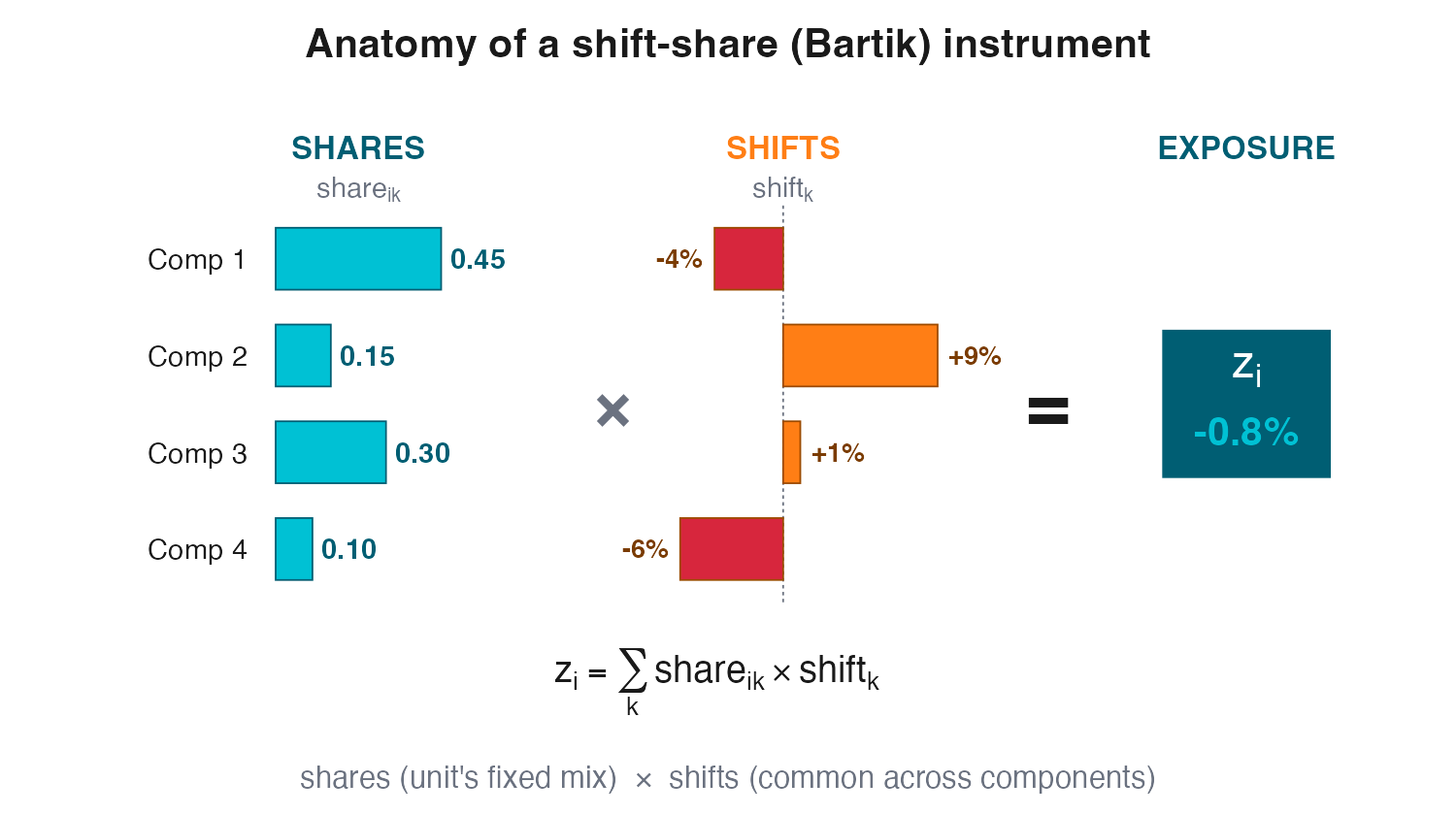
The product \(Z_i = \sum_k s_{ik}\,g_k\) predicts how hard unit \(i\) is hit — without using its own outcome. Exogeneity can live in either piece — shares or shifts. (Bartik 1991)

Introduce the design ABSTRACTLY, before any geography or industries. The instrument projects a set of common component-level shifts \(g_k\) onto each unit through its fixed, pre-period exposure shares \(s_{ik}\), and sums. The product predicts how hard unit \(i\) is “hit” without ever using \(i\)’s own realized outcome — so it can instrument an endogenous treatment \(D_i\) of the same form. Two independent sources of variation are baked in: the shares vary across units, the shifts vary across components — which is exactly why exogeneity can be argued from EITHER side (next slide). Terminology: it is “shift-share”, and \(g_k\) is a “shift” — reserve the word “shock” for a shift you are specifically claiming is exogenous. Bartik (1991) introduced the construction; Goldsmith-Pinkham, Sorkin & Swift and Borusyak-Hull-Jaravel gave the two modern identification foundations. The concrete labor and tech instances come on the next slides.

Where is the exogeneity — in the shares or the shifts?

Validity rests on one of two stories — and you must declare which.

Shares route (Goldsmith-Pinkham, Sorkin, and Swift 2020)

The shares are the instruments (Bartik 2SLS ≡ GMM on the initial shares) — really K stacked difference-in-differences.

Classic: immigrant enclave — an inflow lands in a city through its pre-existing migrant share (Card 2001).

Exogenous if the initial mix doesn’t predict later changes in Y. Rotemberg weights flag the few shares that carry the estimate.

Shifts route (Borusyak, Hull, and Jaravel 2022)

The shifts are as-good-as-random — and many — so the design holds even if the shares are endogenous. SSIV ≡ IV at the shift level.

Classic: the China shock — import growth measured in eight other rich countries purges US-specific demand (Autor, Dorn, and Hanson 2013).

Exogenous if enough independent shifts. Effective sample = # of shifts, not units.

Neither route is free — declare and defend one: a few high-weight shares (Rotemberg), or many, as-good-as-random shifts. Guide: Borusyak, Hull, and Jaravel (2025).

The subtlety students most often miss: shift-share can be valid for two completely DIFFERENT reasons, with different exogeneity tests and different effective sample sizes — so you must declare which. Shares route (Goldsmith-Pinkham, Sorkin & Swift 2020): Bartik 2SLS is numerically GMM that uses the initial shares AS the instruments (their Prop 1.1), so the exclusion restriction is a statement about the SHARES — really K stacked difference-in-differences. The shifts only set the Rotemberg weights (in their canonical labor-supply case the shifts explain <1% of the weight variance). Vivid example: the immigrant ENCLAVE design — an inflow lands in a city through its pre-existing migrant share; identification asks whether that city would have evolved like cities without the enclave. Defend the high-weight shares with pre-trends and correlates. Shifts route (Borusyak, Hull & Jaravel 2022): if the shifts are as-good-as-randomly assigned AND there are many of them, their share-weighted average is itself as-good-as-random — so the design is valid EVEN IF the shares are endogenous, and SSIV equals an IV regression at the SHIFT level. Effective sample = the number of independent shifts (inverse Herfindahl), which can be alarmingly small. Example: the China shock (Autor-Dorn-Hanson 2013) proxies the industry shifts with Chinese import growth in EIGHT OTHER rich countries — stripping out US-specific demand to isolate China-side supply. The classic error is claiming exogeneity for one side casually — and which side actually carries identification depends on the REGIME, it is not a default to the shares. GPSS’s result holds in the few-shifts / many-units case (the canonical Bartik): there the identifying variation concentrates in a handful of shares, so “national shifts are exogenous to any one unit” is not enough — you must defend those high-weight shares (pre-trends, correlates, Rotemberg). BHJ’s result holds in the many-shifts case: there you lean on the shifts and the shares may be endogenous — often the MORE credible story, since shares are equilibrium objects, whenever the shift is externally / quasi-randomly measured (the China shock’s non-US imports; the fansubbing quits). So it is genuinely a choice you argue, not a presumption that shares are exogenous. Borusyak-Hull-Jaravel 2025 is the current practitioner guide; the SE pitfall (the closing slide of this section) follows from the shift-level structure.

Tech shift-share: automation and AI exposure

Same skeleton — a predicted exposure (\(Z\)) instruments the actual, chosen exposure (\(D\)); the shares run over whatever the shift hits — industries (robots) or occupations (AI).

Robots (Acemoglu and Restrepo 2020)

\(D\) (treatment): local robot exposure \(=\sum_k s^{1990}_{\ell k}\,\Delta\text{robots}^{\text{US}}_k\) (\(s\) = a zone’s 1990 industry shares) — endogenous (US adoption tracks industry shocks).

\(Z\) (instrument): the same 1990 industry shares × European adoption \(\Delta\text{robots}^{\text{EU}}_k\) — exogenous (fixed mix, external frontier).

AI (being built now)

\(D\) (treatment): the firm’s actual AI adoption — endogenous (firms adopt on their own prospects).

\(Z\) (instrument): pre-period occupation shares × national AI shock per occupation, \(\sum_o s^{\text{pre}}_{\text{firm},o}\,\text{AI}_o\) — exogenous (fixed mix, external AI wave).

Still IV → still a LATE: a complier-weighted effect, not the effect on every zone or firm.

The family is alive, not historical. Acemoglu & Restrepo’s robot design is the canonical template, and it is a TWO-shift-share IV: the endogenous treatment \(D\) is US robot exposure (1990 industry shares × US robot adoption), and the instrument \(Z\) is the SAME 1990 shares × robot adoption in EUROPE. Why EU adoption instruments US adoption: the same industries are automatable everywhere (autos, electronics, metals robotize in every country; services barely anywhere), so EU adoption is a strong industry-level predictor of US adoption (RELEVANCE) — yet EU firms do NOT respond to US-specific industry-demand shocks, so EU adoption is uncorrelated with the US confounders (EXCLUSION). Mechanically, EU adoption captures the technological-frontier slice of US automation and discards the US-specific demand slice that biases OLS — exactly the ADH “imports in 8 other countries” move. The shares are predetermined (1990, before the robot wave). Threat to exclusion: a common GLOBAL industry shock moving both EU adoption and US local labor markets independent of US robots — defend with industry-characteristic balance and pre-trends. Note the shares run over different DIMENSIONS: robots act on INDUSTRIES, so the shares are a commuting zone’s 1990 industry employment mix; AI acts on OCCUPATIONS/tasks, so the shares are a firm’s pre-period occupation mix — the share is always defined over whatever the shift acts on. The AI analogue is being built now: \(D\) = a firm’s actual AI adoption (endogenous — firms choose); \(Z\) = predicted AI exposure = the firm’s pre-period occupation mix × a national/external AI-exposure shock per occupation (the firm can move neither its historical mix nor the national AI wave). Both are shifts-route (BHJ) bets — the shift is the exogenous part, the shares carry relevance. Two reminders before we leave IV: (1) the AKM SE problem (coming up) applies here too; (2) because this is IV, the estimand is still a LATE — a complier-weighted average, not the effect on every zone/firm.

Shift-share in the wild: fansubbing as copyright infringement

Fansubbing a given anime is endogenous — hits attract subbers. So instrument the supply with a shift-share whose shift is exogenous.

The instrument

\[Z_{a} = \sum_{g} s_{g,a}\,\cdot\,\text{quit}_g\]

\(s_{g,a}\) = group \(g\)’s predicted (pre-period) propensity to sub anime \(a\); \(\text{quit}_g\) = group \(g\) disbands (the shift).

Likely subbers quit → less fansubbing \(D_a\) → effect on legal sales \(Y_a\) (substitution vs. sampling). A shifts-route bet: claim the quits are random, not the shares.

Why a quit can be ~random

Idiosyncratic group deaths: burnout, members graduate, internal drama, a lost translator.

⚠ Killer threat: groups quit because a show got licensed — which moves \(Y\) too. Reverse causation into the shift.

Fixes: predicted (not realized) shares; drop licensing-driven quits; many independent quits.

The professor’s own example, and a perfect “which component is exogenous?” case. Map: unit = anime \(a\); components = fansub groups \(g\); share \(s_{g,a}\) = group \(g\)’s PREDICTED (pre-period) propensity to sub anime \(a\), built only from pre-period features (the group’s historical genre/studio specialization), NEVER the realized subbing of \(a\); shift = group \(g\) disbands. \(Z_a\) = predicted-exposure-weighted loss of fansub capacity; first stage = anime whose likely subbers quit get less/slower fansubbing \(D_a\). This is a BHJ (shifts-exogenous) design: we place NO exogeneity claim on the shares (popular anime have higher propensity) — the entire bet is that the QUITS are as-good-as-random with respect to a given anime’s appeal. Why that can hold: groups die for idiosyncratic, group-level supply reasons — burnout, members graduate/get jobs, internal drama, loss of a key translator/typesetter/encoder — incident to any one title. The killer threat (say it plainly): quitting is a CHOICE. Groups often disband precisely BECAUSE a flagship show got officially licensed (cease-and-desist / “no point continuing”) or lost its fandom — and licensing/popularity also move legal sales \(Y\). That is reverse causation INTO the shift and breaks exclusion. Mitigate by restricting to quits with clearly anime-independent causes and balance-testing \(\text{quit}_g\) against pre-period group characteristics. Other threats: (1) correlated mass-quits — platform crackdowns, tracker shutdowns, licensing waves make many groups quit at once, breaking the many-independent-shifts requirement; absorb with time/season FE. (2) Few relevant groups per anime → tiny effective number of shifts (high Herfindahl); the design then rides on one quit. (3) Rival pickup — when one group quits a popular title another grabs it, so the first stage is weak exactly where demand is high, and the LATE is for the low-demand margin. (4) Predicted-not-realized share is essential: using \(a\)’s realized subbing puts \(D_a\) and \(a\)’s own error inside \(Z_a\) (mechanical first-stage bias) — use a leave-out construction. Cluster/aggregate inference at the GROUP (shift) level, BHJ-style. Outcome \(Y\): official simulcast uptake, speed-to-license, DVD/Blu-ray and legal digital sales — the substitution-vs-sampling question. Verdict: pedagogically excellent for making “defend the shift, not the share” concrete; not a turnkey valid design.

Standard errors are the headline pitfall (AKM)

Shift-share’s most dangerous failure is silent: confident intervals that should not be.

Why naive SEs lie

Regions with similar shares are exposed to the same shocks.

So residuals correlate across regions that may be geographically far apart — geo-clustering misses it entirely.

The fix

Use AKM / AKM0 standard errors (Adão, Kolesár, and Morales 2019).

R package: ShiftShareSE.

Exercise 8 shows it: naive 95% CIs cover only ~60% — AKM/exposure-robust SEs restore them.

The correlation is in exposure space, not geographic space — which is exactly why clustering by state does not save you.

This is the slide that prevents a confident wrong answer. Adao, Kolesar, Morales showed that shift-share residuals are correlated across observations with similar sector shares — even regions on opposite coasts — because they load on the same national shocks. Standard heteroskedasticity-robust or even state-clustered SEs ignore this and dramatically over-reject the null; a “significant” effect can be noise. AKM/AKM0 corrects it; the ShiftShareSE package implements it. The optional Exercise 8 makes this concrete on a simulated shift-share design — naive “95%” CIs cover only ~60% of the time, and exposure-clustering lifts coverage back toward 95%. Emphasize: the bias is in inference, not the point estimate, so it is invisible unless you specifically check for it.

All five so far share one move; the sixth uses a cutoff

Step back: every design in this act borrowed randomness the same way.

Encouragement, lottery, natural experiment, judge-leniency, shift-share — all borrow randomness through a NUDGE Z. The sixth design borrows it at a CUTOFF.

Synthesize the act in one picture. The five designs we just toured are all “nudge” instruments: something shifts the probability of treatment without otherwise touching the outcome — a draw, an invite, a shock, a lenient judge, a predicted exposure. Regression discontinuity is the same logic localized to a threshold: just above and just below a cutoff c, units are as-good-as-randomly on either side. The running variable plays the role of Z, but only right at the boundary. That is the bridge into Act 4 — fuzzy RDD will even reuse our entire 2SLS/LATE apparatus, with the cutoff as the instrument.

RDD: Variation at a Cutoff

Where is the treatment effect on this graph?

Yelp rounds review averages to half-stars — 3.74 → 3.5, 3.76 → 4.0.

Socratic prompt

Two businesses scored 3.74 and 3.76 are essentially identical — yet one rounds up to 4 stars. If the outcome jumps right at the line, what could explain it other than the badge? Hold that thought before we name anything.

Open with no notation at all — just the picture and the question. The on-slide scatter shows the smooth trend and the step at the threshold; ask students to POINT to the jump (the vertical gap between the two fitted lines exactly at the line) and to say why units just-below and just-above are comparable — before any naming. The Yelp half-star example (Anderson & Magruder is the classic) and the LLM-confidence routing threshold are both genuinely “tech” and intuitive. Resist defining “running variable” yet — that is the next slide. Transition: “Let’s give these pieces names.”

The vocabulary, on one running example

Keep the Yelp rating example. One spine, five terms:

Term	In the Yelp example
Running variable \(x\)	underlying review average (continuous)
Cutoff \(c\)	the rounding threshold, e.g. 3.75
Trend \(E[Y\mid x]\)	revenue rises smoothly with reputation
Discontinuity / jump	the step in revenue right at \(c\)
Local regression	a line fit on each side, near \(c\) only

The design’s whole claim: units just below and just above \(c\) are as-good-as-randomly assigned to treatment.

Drip the terms onto the single Yelp spine so nothing feels abstract. Emphasize that x is continuous — that is what makes “just below / just above” meaningful, unlike a binary eligibility rule. The as-good-as-random claim is the bridge back to A/B testing: near the cutoff, the badge is essentially a coin flip determined by noise in the third decimal of the average. Note that “local regression” foreshadows S52 — we never fit one global curve. Transition: “But what exactly is being assumed versus estimated? This is the single most confused point in RDD.”

Smoothness vs discontinuity — identification is NOT estimation

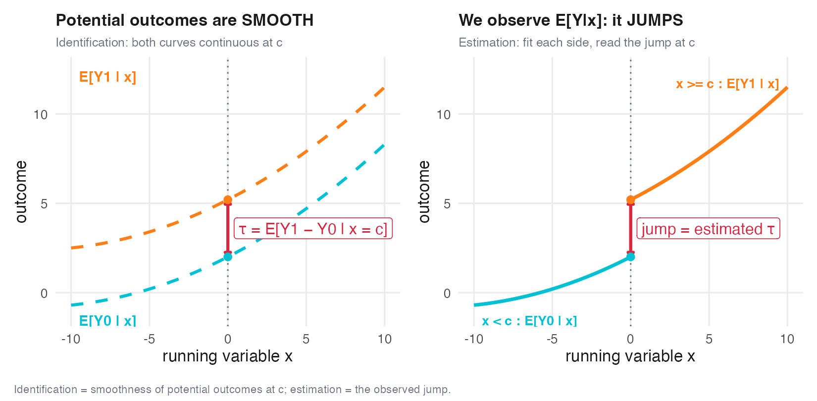
The core distinction

Assumed (unobservable): the potential-outcome curves \(E[Y_0\mid x]\) and \(E[Y_1\mid x]\) are smooth through \(c\) — so that the only thing changing discontinuously at the cutoff is the treatment.

Estimated (observable): the jump in \(E[Y\mid x]\) at \(c\) — what we actually see in the data.

This is THE slide to slow down on. Students conflate the smoothness assumption with the thing they estimate. The assumption is about counterfactual curves we can never see on both sides of c — the dotted continuations. The estimate is a jump in the observed conditional mean. Identification says: IF the unobservable curves are smooth, THEN the observed jump must be the treatment effect, because nothing else changes discontinuously at c. Point at the figure: solid observed curve with a step; faint dotted potential-outcome curves gliding smoothly through. Transition: “When does this give a clean effect? Start with the sharp case.”

Sharp RDD: the jump in E[Y] at c IS the effect

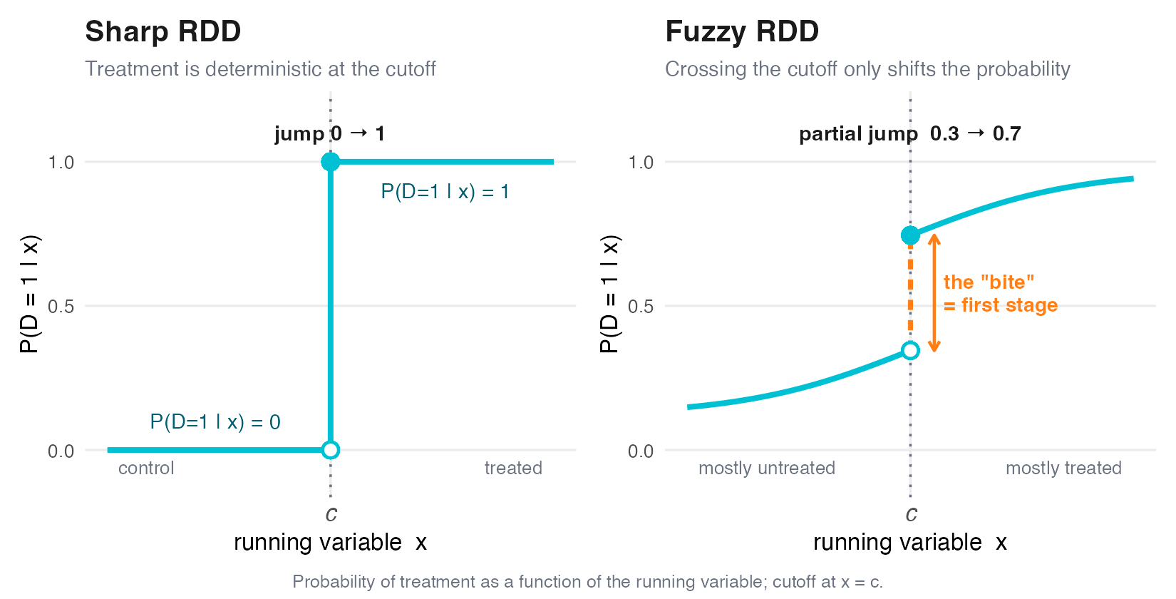
Sharp: treatment switches deterministically at \(c\) (probability \(0 \to 1\)). Then

\[\tau = \lim_{x\downarrow c}E[Y\mid x] - \lim_{x\uparrow c}E[Y\mid x] = E[Y_1 - Y_0 \mid x=c].\]

A treatment effect at the cutoff (Thistlethwaite and Campbell 1960).

Which design? A full \(0\to1\) step in \(E[D\mid x]\) → sharp; a partial jump → fuzzy.

Sharp is the easy case: everyone above c is treated, everyone below is not — no choice, no compliers. The jump in observed E[Y] at c equals the average effect for units sitting exactly at the cutoff. Stress the limits notation: we approach c from both sides and difference. Thistlethwaite and Campbell (1960) invented this studying scholarship awards based on a test-score threshold — sixty-five years old and still the cleanest natural experiment design we have. Transition: “But most real thresholds aren’t sharp — people cross the line and still don’t take the treatment.”

Fuzzy RDD IS a local instrumental-variable design

When crossing \(c\) only changes the probability of treatment, instrument \(D\) with \(Z=\mathbb{1}\{x\ge c\}\):

\[\tau = \frac{\lim_{x\downarrow c}E[Y\mid x] - \lim_{x\uparrow c}E[Y\mid x]}{\lim_{x\downarrow c}E[D\mid x] - \lim_{x\uparrow c}E[D\mid x]} = \frac{\text{jump in } E[Y]}{\text{jump in } E[D]}.\]

Sharp = fuzzy with first stage \(=1\): full step in \(E[D\mid x]\) → sharp; partial → fuzzy.

It is a Wald ratio. Every word from Acts 1–2 carries over, evaluated at the cutoff:

IV concept	Fuzzy-RDD version
Compliers	units who take treatment because they crossed \(c\)
Monotonicity	crossing \(c\) never discourages treatment
Exclusion	\(c\) affects \(Y\) only through \(D\) (smoothness)
Weak instrument	tiny jump in \(E[D]\) ⇒ unstable ratio

Formalized by Hahn, Todd, and Van der Klaauw (2001).

This is the payoff of the whole session — the bridge slide. Fuzzy RDD is not a new method; it is IV where the instrument is “landed on the treated side of the threshold.” The numerator is the reduced-form jump in Y, the denominator the first-stage jump in D — the same Wald ratio as the encouragement design in Act 1. Walk the table left-to-right and watch the relief: compliers, monotonicity, exclusion, weak-instrument all reappear, now localized at c. Hahn, Todd & Van der Klaauw (2001) gave the formal treatment. Transition: “And like every IV, the effect it identifies is LOCAL — in two senses now.”

RDD identifies a LOCAL effect — mind the external validity

What RDD recovers is a LATE at the cutoff — the effect for units sitting right at \(x=c\). Not a global ATE.

A $500 loyalty tier The effect of crossing the $500-spend threshold tells you about customers near $500.

A $5000 tier It says almost nothing about the effect of a premium tier at $5000 — different customers, different margins.

Same caveat, two senses

RDD is local in the complier sense (fuzzy: who responds to crossing \(c\)) and in the covariate sense (only units near \(c\)). Extrapolating to a different threshold is an assumption, not a finding.

The locality is intrinsic to the design (Lee and Lemieux 2010; Imbens and Lemieux 2008).

Mirror the LATE / compliers message from Act 1 so students hear the through-line. RDD gives you a clean effect precisely because it only uses units near c — but that same feature is the external-validity cost. The loyalty-tier example lands for a business audience: a CFO wants the effect of the premium tier, but your data only identifies the entry-tier threshold. Be explicit that extrapolating the cutoff effect to other points on the running variable requires functional-form assumptions you cannot test. Transition: “Given we only trust the data near c, how should we actually fit it?”

Estimate locally — do NOT fit high-order global polynomials

Do: local linear (or quadratic) fit inside a bandwidth around \(c\). Don’t: a single high-order polynomial across the whole range — it is noisy, lets far-away points dictate the fit at \(c\), and miscovers the truth (Gelman and Imbens 2019).

Gelman & Imbens (2019) is the canonical warning: a global cubic or quartic puts wild weight on observations far from the cutoff, and its wiggles near c manufacture spurious jumps. The fix is conceptual, not just mechanical — only data near c is credibly as-good-as-random, so only fit near c. The bandwidth choice (how wide is “near”) is a bias-variance tradeoff we automate in S55. Point at the figure: the global polynomial’s tail-wagging produces a fake discontinuity the local fit does not. Transition: “Local fitting buys credibility only if the design itself is valid — two threats.”

Validity threat 1: did units MANIPULATE the running variable?

If agents can precisely control \(x\) to land on the favorable side, the local-randomization story collapses. Test for a discontinuity in the density of \(x\) at \(c\) (McCrary 2008); modern binning-free version in Cattaneo, Jansson, and Ma (2020).

Caution: density tests can fail spuriously (heaping at round numbers). Use your eyes first, then a donut-hole around \(c\) (drop points at the line, re-estimate).

The intuition: if everyone who barely missed the cutoff could nudge their score up, you’d see a pile-up of units just above c and a hole just below — the density would jump. McCrary (2008) formalized this; Cattaneo, Jansson & Ma (2020) give the binning-free rddensity test we use in the lab. Stress the caution: running variables often heap at round numbers (people report $500 exactly), which trips the test without true manipulation. The donut-hole — drop observations immediately around c — checks robustness to such heaping. Tie it to tech: can a seller game a star average? Can a borrower game a credit score? Transition: “Manipulation is one threat; the other is whether anything else jumps at c.”

Validity threat 2: continuity / placebo checks

The smoothness assumption is partly testable — two placebo-style checks:

Covariate balance Pre-determined covariates (things fixed before treatment) should not jump at \(c\). A jump in, say, prior-year revenue means \(c\) is not as-good-as-random.

Fake cutoffs Run the same RDD at placebo thresholds where nothing happens. There should be no jump at \(c' \neq c\).

Diagnostic checklist for the lab

(1) density of \(x\) at \(c\) (manipulation) · (2) covariate jumps + fake cutoffs (continuity). Same two-threat taxonomy you will run on the FitLife fuzzy-RDD twist.

These mirror the parallel-trends placebos students will meet in S10 difference-in-differences, so flag the recurring logic: you can’t test the identifying assumption directly, but you can test its observable implications. Covariate balance is the RDD analogue of checking baseline balance in an RCT — if treatment near c is really as-good-as-random, predetermined characteristics shouldn’t differ across the line. Fake cutoffs are pure falsification: if your method finds “effects” where none should exist, distrust the real one. Bundle the two threats into one checklist they carry into the lab. Transition: “You don’t hand-roll any of this — there’s tooling that gets the inference right.”

Use the tooling, not hand-rolled OLS

The RDD toolkit

rdrobust — data-driven MSE-optimal bandwidth (CCT, Calonico, Cattaneo, and Titiunik (2014)) plus robust bias-corrected confidence intervals, so the intervals are actually valid (Calonico et al. 2017). rddensity — the manipulation (McCrary-style) test.

A hand-rolled OLS with an arbitrary bandwidth gives a point estimate but invalid standard errors — bias from the local fit leaks into the CI. rdrobust corrects for exactly that.

Mechanics — CCT bandwidth selection, McCrary internals, polynomial order — live in the LAB and NOTES, not this lecture. Practical guide: Cattaneo, Idrobo, and Titiunik (2020).

The headline for a methods audience: the hard part of RDD is not the point estimate, it’s honest inference. Naive local OLS understates uncertainty because the bias of the local polynomial isn’t accounted for in the CI. Calonico, Cattaneo & Titiunik built rdrobust to do MSE-optimal bandwidth selection (CCT 2014) and robust bias-corrected CIs (CCFT 2017) automatically — same authors, same package across R, Stata, and Python. Cattaneo, Idrobo & Titiunik (2020) is the practical guide students can read. Deliberately push the mechanics to the lab so the lecture stays conceptual. Transition: “Where does this show up in a tech business? Almost anywhere there’s a threshold.”

RDD is everywhere tech has a threshold

Threshold	Running variable \(x\) / cutoff \(c\)	Sharp or fuzzy?
Loyalty / rewards tiers	cumulative spend crosses a tier boundary	sharp — auto-enrolled
Ad-auction reserve prices	bid above/below reserve (Ostrovsky and Schwarz 2023)	sharp — mechanical
Search-rank boundaries	relevance score crosses a position cutoff (Narayanan and Kalyanam 2015)	sharp — rule-based
Credit-score gates	FICO crosses an approval threshold	fuzzy — underwriter discretion
Promo eligibility → opt-in	spend / tenure crosses an offer threshold	fuzzy — redemption is partial
Fraud / risk-score review	risk score crosses a review threshold	fuzzy — humans override

RDD recovers a causal effect from logs when no clean A/B test was run — a complement to experimentation, local to the threshold.

Reframe RDD as a default move when you find any rule-based threshold in product logs — and tech is full of them. The third column applies the sharp-vs-fuzzy test: a mechanical gate (tiers, auction reserve, search rank) flips treatment deterministically → sharp; anything gated by discretion or voluntary take-up (credit approval, promo redemption, fraud review) only shifts the probability → fuzzy, so you instrument with the threshold and read a LATE. Ostrovsky & Schwarz (2023) used reserve-price thresholds; Narayanan & Kalyanam (2015) exploited search-rank position cutoffs to measure click effects. The strategic point for a PM or analyst: you didn’t run the experiment, but the business already ran a quasi-experiment for you every time it drew a line. It complements A/B testing rather than replacing it — A/B gives you a global ATE on the randomized population, RDD gives you a clean local effect right at a decision boundary that matters operationally. Transition: “Step back — all six designs this session were one idea.”

Recap: one intuition, six designs, always a LOCAL effect

One idea — find exogenous variation you didn’t assign, then isolate it for a local effect on the units it moves.

Land the unifying arc: every design in this session — classic IV, encouragement, examiner/judge lotteries, shift-share, sharp and fuzzy RDD — is the same move. You locate variation in the treatment that was generated by something other than the unit’s own choice, and you lean on it. The price is always locality: you get the effect on compliers, or on units at the cutoff, never a free global ATE. This consolidates Acts 1–4 before we send them to the lab.

One check protects each design family

Match each design to the one diagnostic that guards it:

Design	Key diagnostic
IV / encouragement / judge	first-stage \(F\) (weak-instrument)
Shift-share (Bartik)	AKM / exposure-robust SEs
RDD (sharp / fuzzy)	McCrary density + bandwidth choice

The diagnostics table is the takeaway artifact — match each design to the one check that protects it: the first-stage F for any instrument, exposure-robust/AKM SEs for shift-share, and the McCrary density test plus bandwidth choice for RDD. Carry this card into the lab. Transition: “Here’s how all of this becomes hands-on.”

To the lab and Assignment III: FitLife, two treatments, one story

The lab uses a synthetic tech DGP: an encouragement IV plus a fuzzy-RDD twist. Assignment III bridges both halves of Part III — the SEND decision with S06 tools and the OPEN decision with S07 tools.

The FitLife storyline runs through S06 and S07: the SEND decision is the confounding problem (you choose whom to email — use matching/IPW/AIPW and sensitivity from S06), while the OPEN decision is the IV problem (you can’t force opens — instrument with the nudge, use 2SLS/LATE/weak-IV from S07). The same synthetic world powers both the lab and Assignment III. Transition: the two decisions answer two different causal questions — that’s the assignment’s payoff.

References

Abdulkadiroğlu, Atila, Joshua D. Angrist, Susan M. Dynarski, Thomas J. Kane, and Parag A. Pathak. 2011. “Accountability and Flexibility in Public Schools: Evidence from Boston’s Charters and Pilots.” Quarterly Journal of Economics 126 (2): 699–748. https://doi.org/10.1093/qje/qjr017.

Acemoglu, Daron, and Pascual Restrepo. 2020. “Robots and Jobs: Evidence from US Labor Markets.” Journal of Political Economy 128 (6): 2188–2244. https://doi.org/10.1086/705716.

Adão, Rodrigo, Michal Kolesár, and Eduardo Morales. 2019. “Shift-Share Designs: Theory and Inference.” The Quarterly Journal of Economics 134 (4): 1949–2010. https://doi.org/10.1093/qje/qjz025.

Anderson, T. W., and Herman Rubin. 1949. “Estimation of the Parameters of a Single Equation in a Complete System of Stochastic Equations.” The Annals of Mathematical Statistics 20 (1): 46–63. https://doi.org/10.1214/aoms/1177730090.

Andrews, Isaiah, James H. Stock, and Liyang Sun. 2019. “Weak Instruments in Instrumental Variables Regression: Theory and Practice.” Annual Review of Economics 11: 727–53. https://doi.org/10.1146/annurev-economics-080218-025643.

Angrist, Joshua D. 1990. “Lifetime Earnings and the Vietnam Era Draft Lottery: Evidence from Social Security Administrative Records.” American Economic Review 80 (3): 313–36. https://www.jstor.org/stable/2006669.

Angrist, Joshua D., Guido W. Imbens, and Donald B. Rubin. 1996. “Identification of Causal Effects Using Instrumental Variables.” Journal of the American Statistical Association 91 (434): 444–55. https://doi.org/10.1080/01621459.1996.10476902.

Angrist, Joshua D., and Alan B. Krueger. 2001. “Instrumental Variables and the Search for Identification: From Supply and Demand to Natural Experiments.” Journal of Economic Perspectives 15 (4): 69–85. https://doi.org/10.1257/jep.15.4.69.

Angrist, Joshua D., and Jörn-Steffen Pischke. 2009. Mostly Harmless Econometrics: An Empiricist’s Companion. Princeton University Press.

———. 2015. Mastering ’Metrics: The Path from Cause to Effect. Princeton, NJ: Princeton University Press.

Arnold, David, Will Dobbie, and Crystal S. Yang. 2018. “Racial Bias in Bail Decisions.” Quarterly Journal of Economics 133 (4): 1885–1932. https://doi.org/10.1093/qje/qjy012.

Autor, David H., David Dorn, and Gordon H. Hanson. 2013. “The China Syndrome: Local Labor Market Effects of Import Competition in the United States.” American Economic Review 103 (6): 2121–68. https://doi.org/10.1257/aer.103.6.2121.

Bartik, Timothy J. 1991. Who Benefits from State and Local Economic Development Policies? Kalamazoo, MI: W.E. Upjohn Institute for Employment Research. https://doi.org/10.17848/9780585223940.

Borusyak, Kirill, Peter Hull, and Xavier Jaravel. 2022. “Quasi-Experimental Shift-Share Research Designs.” The Review of Economic Studies 89 (1): 181–213. https://doi.org/10.1093/restud/rdab030.

———. 2025. “A Practical Guide to Shift-Share Instruments.” Journal of Economic Perspectives 39 (1): 181–204. https://doi.org/10.1257/jep.20231370.

Bound, John, David A. Jaeger, and Regina M. Baker. 1995. “Problems with Instrumental Variables Estimation When the Correlation Between the Instruments and the Endogenous Explanatory Variable Is Weak.” Journal of the American Statistical Association 90 (430): 443–50. https://doi.org/10.1080/01621459.1995.10476536.

Calonico, Sebastian, Matias D. Cattaneo, Max H. Farrell, and Rocío Titiunik. 2017. “Rdrobust: Software for Regression-Discontinuity Designs.” The Stata Journal 17 (2): 372–404. https://doi.org/10.1177/1536867X1701700208.

Calonico, Sebastian, Matias D. Cattaneo, and Rocío Titiunik. 2014. “Robust Nonparametric Confidence Intervals for Regression-Discontinuity Designs.” Econometrica 82 (6): 2295–2326. https://doi.org/10.3982/ECTA11757.

Card, David. 2001. “Immigrant Inflows, Native Outflows, and the Local Labor Market Impacts of Higher Immigration.” Journal of Labor Economics 19 (1): 22–64. https://doi.org/10.1086/209979.

Cattaneo, Matias D., Nicolás Idrobo, and Rocío Titiunik. 2020. A Practical Introduction to Regression Discontinuity Designs: Foundations. Cambridge Elements in Quantitative and Computational Methods for the Social Sciences. Cambridge: Cambridge University Press. https://doi.org/10.1017/9781108684606.

Cattaneo, Matias D., Michael Jansson, and Xinwei Ma. 2020. “Simple Local Polynomial Density Estimators.” Journal of the American Statistical Association 115 (531): 1449–55. https://doi.org/10.1080/01621459.2019.1635480.

Chyn, Eric, Brigham R. Frandsen, and Emily C. Leslie. 2025. “Examiner and Judge Designs in Economics: A Practitioner’s Guide.” Journal of Economic Literature 63 (2): 401–39. https://doi.org/10.1257/jel.20241719.

Cunningham, Scott. 2021. Causal Inference: The Mixtape. Yale University Press. https://mixtape.scunning.com/.

Dobbie, Will, Andres Liberman, Daniel Paravisini, and Vikram Pathania. 2021. “Measuring Bias in Consumer Lending.” The Review of Economic Studies 88 (6): 2799–2832. https://doi.org/10.1093/restud/rdaa057.

Elbers, Benjamin. 2023. “Encouragement Designs and Instrumental Variables for a/b Testing.” Spotify Engineering. 2023. https://engineering.atspotify.com/2023/08/encouragement-designs-and-instrumental-variables-for-a-b-testing.

Farre-Mensa, Joan, Deepak Hegde, and Alexander Ljungqvist. 2020. “What Is a Patent Worth? Evidence from the u.s. Patent ’Lottery’.” The Journal of Finance 75 (2): 639–82. https://doi.org/10.1111/jofi.12867.

Finkelstein, Amy, Sarah Taubman, Bill Wright, Mira Bernstein, Jonathan Gruber, Joseph P. Newhouse, Heidi Allen, and Katherine Baicker. 2012. “The Oregon Health Insurance Experiment: Evidence from the First Year.” Quarterly Journal of Economics 127 (3): 1057–1106. https://doi.org/10.1093/qje/qjs020.

Frandsen, Brigham R., Lars J. Lefgren, and Emily C. Leslie. 2023. “Judging Judge Fixed Effects.” American Economic Review 113 (1): 253–77. https://doi.org/10.1257/aer.20201860.

Gelman, Andrew, and Guido Imbens. 2019. “Why High-Order Polynomials Should Not Be Used in Regression Discontinuity Designs.” Journal of Business & Economic Statistics 37 (3): 447–56. https://doi.org/10.1080/07350015.2017.1366909.

Goldsmith-Pinkham, Paul, Isaac Sorkin, and Henry Swift. 2020. “Bartik Instruments: What, When, Why, and How.” American Economic Review 110 (8): 2586–2624. https://doi.org/10.1257/aer.20181047.

Gordon, Brett R., Florian Zettelmeyer, Neha Bhargava, and Dan Chapsky. 2019. “A Comparison of Approaches to Advertising Measurement: Evidence from Big Field Experiments at Facebook.” Marketing Science 38 (2): 193–225. https://doi.org/10.1287/mksc.2018.1135.

Hahn, Jinyong, Petra Todd, and Wilbert Van der Klaauw. 2001. “Identification and Estimation of Treatment Effects with a Regression-Discontinuity Design.” Econometrica 69 (1): 201–9. https://doi.org/10.1111/1468-0262.00183.

Imbens, Guido W., and Joshua D. Angrist. 1994. “Identification and Estimation of Local Average Treatment Effects.” Econometrica 62 (2): 467–75. https://doi.org/10.2307/2951620.

Imbens, Guido W., and Thomas Lemieux. 2008. “Regression Discontinuity Designs: A Guide to Practice.” Journal of Econometrics 142 (2): 615–35. https://doi.org/10.1016/j.jeconom.2007.05.001.

Kleibergen, Frank, and Richard Paap. 2006. “Generalized Reduced Rank Tests Using the Singular Value Decomposition.” Journal of Econometrics 133 (1): 97–126. https://doi.org/10.1016/j.jeconom.2005.02.011.

Lee, David S., and Thomas Lemieux. 2010. “Regression Discontinuity Designs in Economics.” Journal of Economic Literature 48 (2): 281–355. https://doi.org/10.1257/jel.48.2.281.

Lee, David S., Justin McCrary, Marcelo J. Moreira, and Jack Porter. 2022. “Valid t-Ratio Inference for IV.” American Economic Review 112 (10): 3260–90. https://doi.org/10.1257/aer.20211063.

Manski, Charles F. 2003. Partial Identification of Probability Distributions. Springer Series in Statistics. New York: Springer-Verlag. https://doi.org/10.1007/b97478.

McCrary, Justin. 2008. “Manipulation of the Running Variable in the Regression Discontinuity Design: A Density Test.” Journal of Econometrics 142 (2): 698–714. https://doi.org/10.1016/j.jeconom.2007.05.005.

Montiel Olea, José Luis, and Carolin Pflueger. 2013. “A Robust Test for Weak Instruments.” Journal of Business & Economic Statistics 31 (3): 358–69. https://doi.org/10.1080/00401706.2013.806694.

Narayanan, Sridhar, and Kirthi Kalyanam. 2015. “Position Effects in Search Advertising and Their Moderators: A Regression Discontinuity Approach.” Marketing Science 34 (3): 388–407. https://doi.org/10.1287/mksc.2014.0893.

Ostrovsky, Michael, and Michael Schwarz. 2023. “Reserve Prices in Internet Advertising Auctions: A Field Experiment.” Journal of Political Economy 131 (12): 3352–76. https://doi.org/10.1086/725702.

Sharma, Amit, Jake M. Hofman, and Duncan J. Watts. 2015. “Estimating the Causal Impact of Recommendation Systems from Observational Data.” In Proceedings of the Sixteenth ACM Conference on Economics and Computation (EC ’15), 453–70. https://doi.org/10.1145/2764468.2764488.

Staiger, Douglas, and James H. Stock. 1997. “Instrumental Variables Regression with Weak Instruments.” Econometrica 65 (3): 557–86. https://doi.org/10.2307/2171753.

Stock, James H., and Motohiro Yogo. 2005. “Testing for Weak Instruments in Linear IV Regression.” In Identification and Inference for Econometric Models: Essays in Honor of Thomas Rothenberg, edited by Donald W. K. Andrews and James H. Stock, 80–108. Cambridge: Cambridge University Press. https://doi.org/10.1017/CBO9780511614491.006.

Thistlethwaite, Donald L., and Donald T. Campbell. 1960. “Regression-Discontinuity Analysis: An Alternative to the Ex Post Facto Experiment.” Journal of Educational Psychology 51 (6): 309–17. https://doi.org/10.1037/h0044319.

Thank you for your attention!
	www.startupengineer.io/team/ihl/ christoph-ihl christophihl