Online A/B testing is causal inference at industrial scale: Microsoft, Netflix, and DoorDash each run tens of thousands of experiments per year, and the methods they have invented to handle that volume — CUPED, anytime-valid sequential tests, switchback designs, and Bayesian decision rules — are now the field’s modern toolkit. This session shows that S04’s blocking is the same thing as tech-industry stratified A/B testing, introduces CUPED and its ML extensions (CUPAC, MLRATE, CURE) as Lin-(2013) adjustment with the pre-period outcome, and then resolves the two open promises from S04: Fisher’s permutation logic becomes A/B-test p-values, and the Bayesian credible interval becomes the proper cure for the frequentist CI misreadings. The session closes with what breaks when textbook A/B assumptions fail — sample ratio mismatch, SUTVA violations in marketplaces, and the switchback designs that DoorDash and Lyft use to handle them — and a surrogate-index slide showing the limits of “long-horizon decisions on short-horizon proxies.” The PBL session works through five progressive exercises spanning all five stacks; Exercise 5 (SRM diagnostic) directly prepares the Quiz II material that gates Assignment II.
7.3 Lecture Notes
7.3.1 Online A/B at scale, OEC, and metric design
7.3.1.1 Why tech firms run tens of thousands of experiments
Bing once attributed a $100M per year annual revenue lift to a single ad-layout experiment that a junior engineer had built on a slow afternoon (Kohavi, Tang, and Xu 2020, ch. 1). Across Microsoft, Booking, Netflix, LinkedIn, and Airbnb the modal experiment outcome looks nothing like that: Kohavi’s “1/3, 1/3, 1/3” rule of thumb says that roughly one third of features ship with a positive effect, one third are flat, and one third hurt the OEC and must be reverted. Stated more bluntly: about 85% of product-team hypotheses fail to ship as proposed. That asymmetry — the rare blockbuster, the routine bust — is precisely why platform-scale experimentation pays off. The expected value of a single feature is small and noisy; the expected value of a pipeline that screens hundreds of features per quarter through a trustworthy A/B platform is enormous.
The implication for this course is operational: the techniques in S04 (random assignment, OLS with HC-robust SEs, Lin adjustment) are necessary but not sufficient. Once experiments run continuously, in parallel, on millions of users, new failure modes appear that textbook RCTs never had to confront — and new tools exist to handle them. 4 put it directly: online controlled experimentation creates statistical challenges that are not encountered in traditional applications, and the unprecedented scale at which experimentation is now conducted in industry has driven much of the recent innovation in this area. The rest of this session catalogues those tools.
7.3.1.2 The OEC is the single most important metric-design decision
Every A/B platform forces one decision before the first user is randomized: which single number defines winning? Kohavi calls this the Overall Evaluation Criterion (OEC) (Kohavi, Tang, and Xu 2020, ch. 7). A good OEC is
Singular: one number per experiment, not a dashboard of 50;
Long-term aligned: maximising it over a 6-month window should advance the business goal, not just the experiment’s immediate metric;
Fast-feedback: must be measurable inside the typical 1–4 week experiment window, otherwise it cannot gate decisions.
Around the OEC sit two supporting tiers. Driver metrics are the secondary numbers an analyst inspects when the OEC moves (clicks per session, time on page, scroll depth). Guardrail metrics are the constraint metrics that block a launch even when the OEC improves: page-load time, crash rate, error rate, complaint volume. Data-quality metrics are the diagnostic layer — sample-ratio mismatch percentage, missing-data fraction, instrumentation-error counts — that decide whether the experiment is even interpretable.
NoteWhat an OEC is NOT
The OEC is not a P&L line. Quarterly revenue is too slow, too lagged, and too easily moved by exogenous shocks to gate a 14-day A/B test.
The OEC is not a single ML loss. Validation cross-entropy is an engineering target for model training; user-experienced behaviour — sessions per user, conversion to paid plan — is the causal target the experiment is testing.
The OEC is not a vanity metric. “Daily active users” goes up when you spam push notifications; sessions-per-user goes down when the spam annoys people. The OEC must be the user-aligned metric, not the one that flatters the launch deck.
The OEC is not immutable. Healthy organisations refresh the OEC quarterly as the business model evolves: a subscription service’s OEC differs from an ad-supported service’s, and a marketplace’s differs from both.
7.3.1.3 Internet-search OEC: queries-per-user vs. sessions-per-user
The cleanest example from Kohavi ch. 7 makes the OEC-design point viscerally: a search engine could plausibly optimise for queries per user, on the logic that more queries = more user engagement = more ad inventory. But a user typing five queries in a row before clicking a result is failing to find what they want. The metric that aligns with the long-term business is sessions per user — the user came back tomorrow because today’s session resolved their need. Optimising queries-per-user can directly destroy sessions-per-user; the wrong OEC choice ships features that look good on the launch dashboard and erode user retention over the following months. Once you have lived through one of those mistakes, you stop arguing about the OEC and start fighting for it.
7.3.1.4 The “Five Puzzling Outcomes” warn that operational details matter
The OEC framework would not exist if not for a corpus of painful experiences. 15 documented five real Bing experiments whose headline results were ultimately driven not by the feature change itself but by operational artefacts: click-tracking failures inflating treatment metrics, primacy effects that decayed over the first week, carryover from a prior experiment running on the same users, and an analysis that ignored the experiment’s actual sample-ratio mismatch. The lesson is uncomfortable: at platform scale, most “interesting” results are wrong before they are interesting. The five puzzles motivate the diagnostic discipline of when A/B breaks (Twyman’s law, SRM checks, SUTVA, surrogate-index caveats); they also explain why modern A/B platforms ship with extensive automated guardrails rather than treating the analyst’s judgment as the last line of defence.
A direct continuation lives in 17, who replicate the 55% click-through-rate lift reported in 16 Study 2 (rounded vs. sharp CTA buttons on an e-commerce homepage; \(n = 919\) visits, \(p = 0.037\)). Three pre-registered replications at SeaWorld and Coop Norway — with 2.8M, 2.2M, and 1.9M users (each over 2,000× the original sample) — returned estimated lifts of 0.16% (\(p = 0.20\)), 0.29% (\(p = 0.60\)), 0.73% (\(p = 0.09\)): two orders of magnitude smaller, all 95% confidence intervals containing zero. BAC’s Study 2 was simply under-powered: no pre-declared MDE, no power calculation, and a 919-visit sample in a domain where real effects sit well under 1%. (Their companion Study 1 had separate problems — a 44:56 sample-ratio mismatch with \(z = 46\), plus Google Ads’ non-random assignment — but the +55% headline came from Study 2, not Study 1.) The winner’s-curse mechanism explains the 55% perfectly: any underpowered study that produces a “significant” result must have over-estimated the true effect (the rejected hypotheses include the smaller, true effects). When tens of thousands of experiments run per year, even tiny SRM rates produce a steady stream of plausible-looking false positives. The operational moral is that good A/B platforms automate the diagnostics, and good experimenters declare an MDE and power before the test starts.
7.3.2 Stratified A/B and CUPED
This stack cashes the S04 forward pointer: stratified A/B testing is blocked randomization with tech-industry vocabulary. Microsoft’s ExP, Netflix’s experimentation platform, Booking, LinkedIn’s XLNT, and Uber’s Morpheus all stratify on the same kinds of features S04’s blocked-RA estimator handled — activity decile × market × device, country × plan × pre-period-minutes, platform × device × country, and so on. The estimator is unchanged from S04:
with \(S_k\) indexing the strata and \(\pi_k\) their relative size. Exercise 1 reapplies the S04 Exercise 3 simulation under this jargon, confirming the variance ratio is identical.
7.3.2.1 CUPED is Lin (2013) with the pre-period outcome as the covariate
CUPED — Controlled-experiment Using Pre-Experiment Data(Deng et al. 2013) — is the analysis-stage cousin of stratification. Instead of designing the randomization to balance on a pre-period covariate, CUPED leaves the randomization alone and adjusts the outcome at analysis time using the pre-experiment outcome\(Y^{\text{pre}}\). The estimator is one line:
The ATE is then estimated by the difference of group means on \(Y^{\text{cuped}}\). The variance of the adjusted outcome shrinks by a factor of \((1 - \rho^2)\) where \(\rho = \text{Cor}(Y, Y^{\text{pre}})\):
A small algebra check: \(\text{Var}(Y^{\text{cuped}}) = \text{Var}(Y - \theta Y^{\text{pre}}) = \text{Var}(Y) - 2\theta\,\text{Cov}(Y, Y^{\text{pre}}) + \theta^2 \text{Var}(Y^{\text{pre}})\). Plug in the optimal \(\theta = \text{Cov}(Y, Y^{\text{pre}})/\text{Var}(Y^{\text{pre}})\) and the second and third terms combine to \(-\text{Cov}(Y, Y^{\text{pre}})^2 / \text{Var}(Y^{\text{pre}}) = -\rho^2 \text{Var}(Y)\), giving the \((1 - \rho^2)\) result.
The connection to S04 is immediate: setting \(X^{\text{pre}} = Y^{\text{pre}}\) in 2’s interaction estimator (with mean-centred covariates) reproduces CUPED with a single regression. CUPED is Lin (2013), specialised to the single-covariate case where the covariate is the pre-experiment outcome. The reason CUPED is presented as a separate method is operational: production platforms apply the \(\theta\)-adjustment in a single pass over a pre-computed \(Y^{\text{pre}}\) table, which is much cheaper than fitting per-experiment interaction OLS at petabyte scale.
The Microsoft headline number: \(\rho \approx 0.7\) for typical engagement metrics, giving \(\text{Var}(Y^{\text{cuped}}) / \text{Var}(Y) \approx 1 - 0.49 \approx 0.51\) — roughly a 50% variance reduction, which under the standard \(n \propto 1/\text{Var}\) scaling translates into 2× experiment throughput per quarter at fixed power (Deng et al. 2013). Microsoft attributes the doubling of Bing’s experimentation velocity post-2013 to the rollout of this single technique.
7.3.2.2 ML extensions: CUPAC, MLRATE, CURE
CUPED’s pre-period outcome is only one of many predictors of \(Y\). Three production extensions push further.
CUPAC — DoorDash’s “Control Using Predictions As Covariates” — replaces \(Y^{\text{pre}}\) with a gradient-boosted regression prediction\(\hat f(X^{\text{pre}})\) trained on a rich set of pre-period features (user activity decile, market, device, hour-of-day patterns, prior-week order counts). When the predictor explains substantially more variance than the raw \(Y^{\text{pre}}\) alone, the residual variance shrinks further and the SE drops. DoorDash reports approximately 40% additional test-length reduction on top of CUPED in their production rollout (DoorDash Engineering Blog, “Improving Experimental Power Through Control Using Predictions As Covariates”). The estimator is still unbiased under random assignment for the same reason CUPED is: \(\hat f(X^{\text{pre}})\) is a function of pre-treatment variables and is therefore exogenous to \(D\).
MLRATE — Machine Learning Regression-Adjusted Treatment Effect(Guo et al. 2021) — is the academically-grounded version. It uses cross-fitting and a doubly-robust adjustment to remain unbiased even when the ML predictor is misspecified. On 48 Facebook metrics, MLRATE reported variance reductions of up to 70%; the cross-fitting machinery directly previews S08’s Double Machine Learning treatment of nuisance functions. The cost is operational complexity — one extra training pass per experiment per cross-fitting fold.
CURE — Statsig’s April 2025 release — builds on CUPED with a non-parametric residual model that captures non-linear relationships between \(Y^{\text{pre}}\) and \(Y\). Statsig reports 10–20% additional variance reduction on top of CUPED on its production traffic (“Announcing CURE”, Statsig Engineering Blog, 2025). The method is recent and not yet peer-reviewed; flag accordingly when citing in coursework.
7.3.2.3 CUPED design checklist
(Kohavi, Tang, and Xu 2020, ch. 22) gives the practitioner discipline. Three items must hold for CUPED to be valid and effective.
Pre-period length. One to two weeks of pre-experiment data is the standard. Shorter pre-periods leave \(Y^{\text{pre}}\) too noisy to be a useful predictor; longer pre-periods add data that is decreasingly correlated with the experiment-period outcome.
\(\theta\) refresh cadence. Re-estimate \(\theta\) at the start of each new experiment, not per-day during the experiment. Updating \(\theta\) during the experiment introduces a feedback loop between the adjustment weight and the realised treatment-effect estimate, which can bias the SE.
Pre-treatment validity. The pre-period for unit \(i\) must precede the treatment assignment for unit \(i\). The standard mistake is to apply CUPED to users who joined the platform after randomization, where “pre-period” includes treated-period data — a classic post-treatment-conditioning bug that re-introduces bias.
The closing punchline: variance reduction is experimental throughput. Every method in this stack converts variance into more experiments per quarter; CUPED’s ~50% conversion is the well-trodden floor, and CUPAC / MLRATE / CURE push further when the operational cost is justified.
7.3.3 Three inference modes
S04 left two threads dangling. The first was Fisher’s randomization test from the previous session, which we said would return next session as the engine of A/B-test p-values. The second was the previous session’s table of CI misinterpretations, which we said would be cured by the Bayesian credible interval introduced here. Both promises close in this stack.
7.3.3.1 Fixed-horizon inference and minimum detectable effect
The textbook A/B test of S04 is the fixed-horizon mode: declare a target sample size \(n^*\) before the experiment starts, run until \(n = n^*\), run a single two-sided t-test (or HC-robust OLS) on the OEC, and decide. The t-test mechanics are unchanged from the previous session’s hypothesis-testing procedure; the new question is how to choose \(n^*\) in the first place.
The minimum detectable effect (MDE) framework gives the answer. Suppose we want to detect a true effect of size \(\delta\) at significance level \(\alpha\) (typically 0.05) with power \(1 - \beta\) (typically 0.80). The required per-arm sample size is
where \(\sigma^2\) is the within-arm variance of the OEC. With \(\alpha = 0.05\) (so \(z_{\alpha/2} = 1.96\)) and \(\beta = 0.20\) (so \(z_\beta = 0.84\)), the numerator’s \(z\)-sum is \(2.80\), and \(n \approx 15.7 \,\sigma^2 / \delta^2\) per arm. For a metric with coefficient of variation \(\sigma/\mu = 2\) and a target relative lift of 1% (\(\delta = 0.01\mu\)), plugging in \(\sigma^2/\delta^2 = 4\mu^2/(0.01\mu)^2 = 40{,}000\) gives roughly 627,000 users per arm (~1.25M total). This is why platform-scale \(n\) in the high six figures or low millions is normal: tiny relative effects on noisy engagement metrics demand exactly this much data — and the variance-reduction methods are how teams compress the requirement. R’s pwr::pwr.t.test() and Python’s statsmodels.stats.power.tt_ind_solve_power() invert the formula for you.
Two practical consequences. First, power is a planning tool, not a result: report it before the experiment starts, not after. Second, do not pre-emptively halt the experiment before reaching \(n^*\) just because an early-looking effect “looks good.” That move is the peeking pathology, and the fixed-horizon machinery is mathematically defenceless against it.
The Fisher permutation test — the permutation / Fisher randomization test from the previous session — is the second move here. The permutation test you saw last session is exactly the engine of Optimizely’s exact A/B p-values. When the classical t-test assumptions fail — small \(n\), heavy-tailed outcomes, contaminated metrics — modern A/B platforms (Optimizely, VWO) fall back to a Monte Carlo Fisher randomization test that produces an exact finite-sample p-value: re-shuffle the treatment labels \(B\) times, compute \(\hat\tau_\pi\) on each shuffle, report the fraction with \(|\hat\tau_\pi| \geq |\hat\tau_{\text{obs}}|\). The S04 Fisher slide and this fixed-horizon block are the same procedure, packaged for two different audiences.
7.3.3.2 The peeking pathology
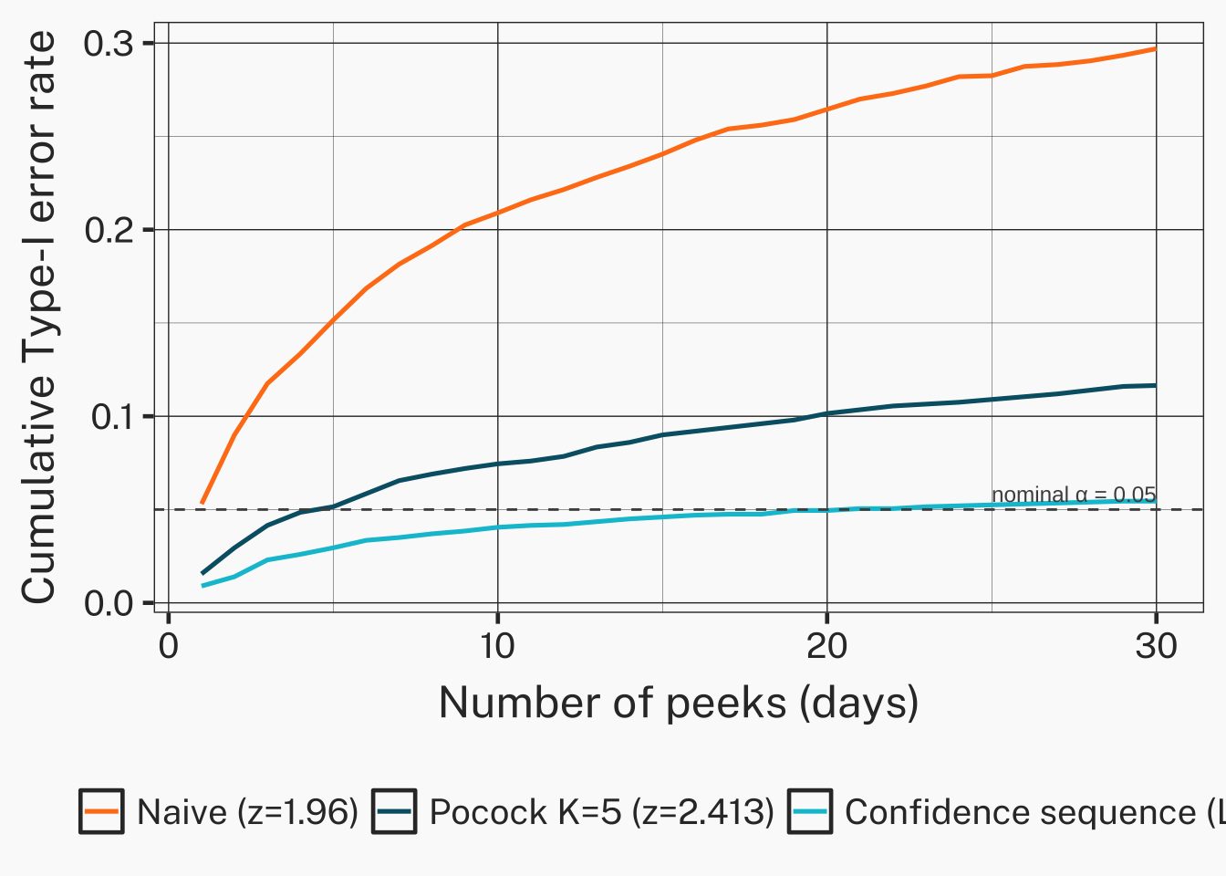
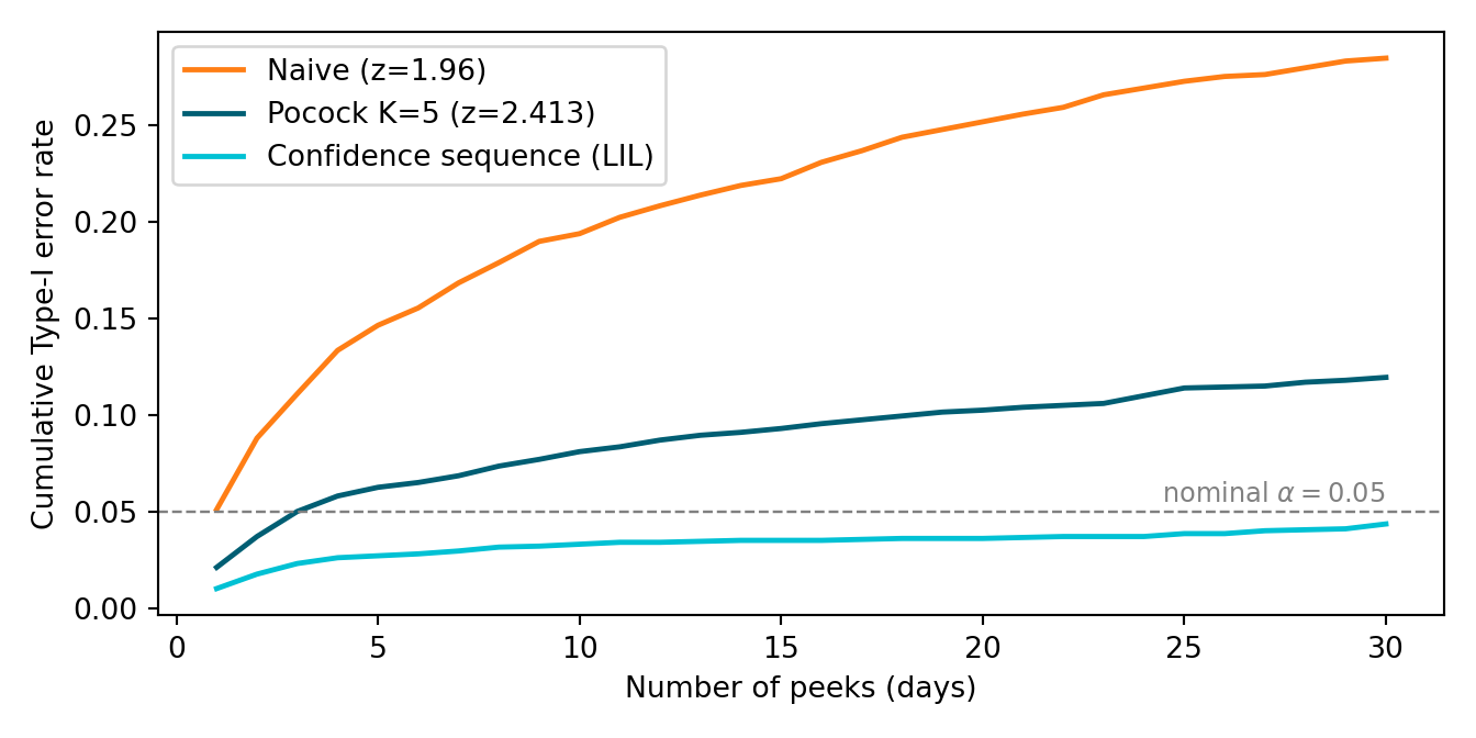
Suppose you set up a fixed-horizon A/B test with \(\alpha = 5\%\) but, because the dashboard updates daily, you give yourself permission to “stop early if the result looks definitive.” Each day’s t-test, viewed in isolation, has Type-I rate 5%. The probability that at least one of 30 daily tests rejects under the null is much higher — in the dependent-test setting of an A/B platform, simulations show the cumulative false-positive rate at 30 daily peeks is roughly 30%. The five-, ten-, and thirty-day curves climb steeply: about 14% at five peeks, 22% at ten, 30% at thirty.
The peeking pathology is not academic. 7 ran a field study on 4,964 A/B tests at a major online marketplace and found that 28–37% of nominally significant results were false discoveries — a direct consequence of peeking and selective stopping interacting with the marketplace’s continuous-monitoring dashboard.
The simulation below reproduces the inflated rate empirically. Run a moderate number of null-hypothesis A/B tests, check daily for 30 days, count the fraction where any peek rejects at \(p < 0.05\).
set.seed(2026)peeks <-30n_per_arm_per_peek <-50trials <-500# bump to 10,000 for the headline ~30% on a fast machineany_reject <-vapply(seq_len(trials), function(i) { reject <-FALSE Yt <-numeric(0); Yc <-numeric(0)for (k inseq_len(peeks)) { Yt <-c(Yt, rnorm(n_per_arm_per_peek)) Yc <-c(Yc, rnorm(n_per_arm_per_peek))if (t.test(Yt, Yc)$p.value <0.05) { reject <-TRUE; break } } reject}, logical(1))mean(any_reject)
[1] 0.294
import numpy as npfrom scipy import statsrng = np.random.default_rng(2026)peeks, n_step, trials =30, 50, 500# bump trials to 10,000 for headline ~30%any_reject = np.zeros(trials, dtype=bool)for i inrange(trials): Yt, Yc = np.empty(0), np.empty(0)for k inrange(peeks): Yt = np.concatenate([Yt, rng.normal(size=n_step)]) Yc = np.concatenate([Yc, rng.normal(size=n_step)])if stats.ttest_ind(Yt, Yc).pvalue <0.05: any_reject[i] =Truebreakprint(round(any_reject.mean(), 3))
0.256
The reported fraction will land in the 0.20–0.30 range at trials = 500; bumping to trials = 10000 tightens it on the headline ~0.30 number. One nominal 5% test, run 30 times with early stopping, becomes a 30% test in practice.
7.3.3.3 Sequential and anytime-valid testing
The peeking pathology has three modern cures: alpha-spending boundaries, sequential / anytime-valid confidence sequences, and Bayesian decision rules. The latter two are this stack’s main material.
A confidence sequence\(\{C_n\}_{n \geq 1}\) is a sequence of intervals with the time-uniform coverage property
Compare this to a fixed-horizon CI, which has \(\Pr(\theta \in C_{n^*}) \geq 1 - \alpha\) for one specific \(n^*\) chosen in advance. The confidence sequence permits stopping at any \(n\) while preserving the family-wise error rate — it is, by construction, peeking-safe (Howard et al. 2021).
9 derive an especially tight family of confidence sequences by re-framing inference as a betting game: at each new observation, an imaginary gambler places a fractional bet against the null. Their accumulated wealth is a non-negative martingale, and Ville’s inequality translates the wealth into an anytime-valid \(p\)-value. Inverting the procedure — collecting the set of candidate parameter values whose wealth process has not yet exceeded \(1/\alpha\) — gives a confidence sequence that is typically 20–40% tighter than the mixture-supermartingale bounds of 8 on bounded outcomes. Both constructions are production-ready in the confseq R package and betting-cs Python implementations.
Sequential is now the industry default. As of 2026, Eppo, Statsig, and Optimizely all ship sequential-by-default; fixed-horizon is the opt-in mode. The reversal is recent — as recently as 2020, fixed-horizon was the default and sequential was an “advanced” option. The Berman & Van den Bulte 2022 false-discovery evidence drove the shift. Microsoft ExP is the lone holdout among major vendors, still defaulting to fixed-horizon with planned-look alpha-spending (a legacy of its 2007 internal design).
Sequential CSs are not free. At the planned sample size \(n^*\), a confidence sequence is typically 15–25% wider than the fixed-horizon CI at the same \(n^*\) — the law-of-iterated-logarithm correction that any anytime-valid procedure must pay (the half-width scales as \(\sqrt{2 \log \log n / n}\) instead of \(1/\sqrt{n}\)). The honest trade-off: if you genuinely run a one-shot experiment with no monitoring, fixed-horizon delivers a tighter interval. If you’re going to monitor and may stop early, the peeking-freedom more than pays for the extra width, since you typically stop well before \(n^*\).
Netflix Sequential is the production capstone. 10 unify the two threads of this deck — variance reduction (Stack 2) and anytime-valid inference (this stack) — into a single estimator: the CUPED-adjusted residual \(Y^{\text{cuped}}\) feeds into a betting confidence sequence that the experimenter can monitor without peeking penalty. The Netflix Tech Blog “Sequential Testing at Netflix” Pt. 1 (continuous outcomes) and Pt. 2 (counting processes for clicks/conversions) walk through the production code, including the bias-correction term that the CUPED residual introduces into the martingale construction. The operational payoff: variance reduction and sequential testing compound multiplicatively. CUPED halves variance; sequential testing eliminates the peeking penalty. Together they reduce time-to-decision by ~4× versus naïve fixed-horizon analysis.
7.3.3.4 Bayesian A/B testing
The previous session’s table of CI misinterpretations gave you the four-row CI-misreadings table: students consistently want frequentist CIs to deliver direct probability statements about the parameter, and the frequentist machinery refuses. The Bayesian credible interval is the cure. Here is the three-column version that completes the S04 contract.
NoteWhat people want a CI to mean –> what it actually means –> what the Bayesian reading delivers
What people want
What the frequentist CI actually says
The Bayesian reading you wanted
“\(p = 0.03\) means there’s a 3% chance the null is true.”
\(p\) is \(\Pr(\text{data} \mid H_0)\), not \(\Pr(H_0 \mid \text{data})\).
\(\Pr(H_0 \mid \text{data})\) is the posterior probability of the null; with a uniform prior on \(\theta_A - \theta_B\), you compute it directly from posterior draws.
“There’s a 95% chance the true \(\beta_1\) lies in this CI.”
Across hypothetical re-samples, 95% of constructed intervals cover \(\beta_1\).
The 95% credible interval\([L, U]\) satisfies \(\Pr(\theta \in [L, U] \mid \text{data}) = 0.95\) by construction. The intuitive reading is literally correct under the posterior.
“\(\alpha = 0.05\) is the probability I’m wrong.”
\(\alpha\) is the long-run Type-I error rate of the procedure.
The expected loss decision rule replaces \(\alpha\): compute \(\mathbb{E}[\text{loss of wrong decision} \mid \text{data}]\) from the posterior and ship if it falls below a business-set threshold \(\varepsilon\).
“A non-significant result means \(H_0\) is true.”
Only “no detectable effect at this \(n\) and \(\alpha\).”
The posterior on \(\theta\) quantifies how much mass is at or near zero; “consistent with no effect” is a posterior-mass statement, not a procedural one.
The mechanics are old and clean. For a binary conversion-rate experiment with \(\theta_A\) and \(\theta_B\) the per-arm true conversion rates, the Beta-Binomial conjugate gives a closed-form posterior. With a uniform \(\text{Beta}(1, 1)\) prior and \(s_j\) successes from \(n_j\) trials in arm \(j\), the posterior is \(\theta_j \mid \text{data} \sim \text{Beta}(1 + s_j, 1 + n_j - s_j)\) — where \(s_A\) = observed conversions in arm A, \(n_A\) = users in arm A (likewise for B). Draw \(M = 100{,}000\) samples from each marginal posterior and compute \(\Delta^{(m)} = \theta_B^{(m)} - \theta_A^{(m)}\). The posterior probability that B beats A is the empirical fraction of \(\Delta^{(m)} > 0\); the 95% credible interval is the empirical 2.5%–97.5% quantile range of \(\Delta^{(m)}\).
The expected-loss decision rule ships only when the cost of being wrong is small enough. Define the loss of shipping B when A is actually better as \(\text{loss}(B \text{ over } A) = \max(\theta_A - \theta_B, 0)\). The posterior expected loss is \(\mathbb{E}[\max(\theta_A - \theta_B, 0) \mid \text{data}] \approx \frac{1}{M} \sum_m \max(\theta_A^{(m)} - \theta_B^{(m)}, 0)\). The decision rule is: ship B if expected loss < \(\varepsilon\), where \(\varepsilon\) is a business-set threshold calibrated to the metric scale (for absolute conversion rates around 6%, \(\varepsilon = 10^{-4}\) is the Eppo/Statsig default; for relative-lift metrics, \(\varepsilon \approx 0.005\) of baseline is more common). Both vendors implement this as the default Bayesian decision rule.
TipWorked example: a high \(P(B > A)\) does not imply ship
The lecture slide for this rule runs the example on \(n_A = n_B = 12{,}000\) with \(s_A = 720\), \(s_B = 762\) (≈ 6.0% vs. 6.35% conversion). At set.seed(2026) the posterior gives \(P(\theta_B > \theta_A \mid \text{data}) \approx 0.87\) — a confident-sounding lead — but the expected loss is
Decompose it: the ≈ 13% of posterior mass where B is worse contributes an average gap of ≈ 0.0016 (i.e., ≈ 0.16 pp of conversion rate), and \(0.13 \times 0.00159 \approx 2.06 \times 10^{-4}\). That exceeds \(\varepsilon = 10^{-4}\), so the rule says do not ship B yet — keep collecting data until either \(P(B > A)\) climbs (shrinking the 13% factor) or the posterior tightens (shrinking the 0.16 pp factor). The lesson: high posterior probability of being best is not the same as low expected regret. Expected loss combines probability and magnitude.
Exercise 4 walks through the full Beta-Binomial / expected-loss / decision-rule pipeline on the same conversion-rate scenario (Kohavi, Tang, and Xu 2020, ch. 17). The three modes side by side. Fixed-horizon \(p\)-values, confidence sequences, and Bayesian credible intervals answer different questions: fixed-horizon delivers \(P(\text{data} \mid H_0)\) at a single pre-committed \(n\) and is not peeking-safe; confidence sequences deliver \(P(\theta \in C_n \;\forall n) \geq 1 - \alpha\) and are peeking-safe by construction, at the cost of 15–25% wider intervals; credible intervals deliver the direct \(P(\theta \in [L,U] \mid \text{data}) = 0.95\) statement and are coherent under any stopping rule, with widths roughly matching fixed-horizon under a flat prior. A decision heuristic: pre-committed one-shot launches (regulatory submission, single launch gate) → fixed-horizon for tightness; continuously-monitored experiments → sequential for peeking-safety; multi-armed asymmetric-cost decisions → Bayesian expected loss. In 2026 tech, sequential is the safe default ~80% of the time; Bayesian is gaining ground in conversion-rate testing; fixed-horizon survives in regulated industries.
7.3.4 When A/B breaks
Even with a perfect OEC, a tuned CUPED, and a sequential-valid inference mode, the textbook A/B contract fails in four distinct ways. Each is a separate diagnostic.
7.3.4.1 Sample Ratio Mismatch (SRM)
A sample ratio mismatch is a discrepancy between the intended assignment ratio (typically 50/50) and the observed count of users in each arm. SRMs occur in roughly 6% of Microsoft A/B tests and 10% of LinkedIn’s zoomed-in / opt-in tests (Fabijan et al. 2019). Causes: bot filtering applied asymmetrically across arms, redirect failures that drop one arm’s users at the load balancer, late-binding instrumentation that misses early-treated users, opt-out flows that disproportionately exit one arm. The diagnostic is a chi-squared test on the observed counts against the intended ratio:
The Kohavi threshold for action is p < 0.001(Kohavi, Tang, and Xu 2020, ch. 21). When SRM is detected, the only correct response is to stop and debug the pipeline. Do not interpret the experiment’s headline result — the bias from differential dropout almost always exceeds the apparent effect size, and reporting a “winner” from an SRM’d experiment is the single most common form of A/B malpractice. Exercise 5 trains exactly this diagnostic on three datasets with intended 50/50 splits but different observed deviations.
7.3.4.2 SUTVA violations and interference
The Stable Unit Treatment Value Assumption (SUTVA) says unit \(i\)’s outcome depends only on unit \(i\)’s treatment — \(Y_i = Y_i(D_i)\), not \(Y_i(D_1, \ldots, D_n)\). Three canonical violation patterns in tech:
Ride-share: surge pricing for treated riders displaces untreated riders’ wait times via the shared driver pool.
Marketplace: a new search ranking shifts shared supply between treated and untreated buyers — treated buyers absorb listings that would have matched untreated buyers in the same geo/category.
Social network: a feed-ranking change reaches untreated users via friend activity (likes, shares, re-posts surfaced in their own feeds).
In each case, \(Y_i\) depends on \(D_j\) for some \(j \neq i\) — SUTVA fails. The DAG has cross-arrows \(D_i \to Y_j\) and \(D_j \to Y_i\) for any pair \(i, j\) sharing a market, a feed, or a supply pool. User-level randomization estimates an effect diluted by spillover — usually toward zero in two-sided marketplaces (untreated users absorb part of the treatment’s positive externality), occasionally away from zero (e.g., when the treatment cannibalises a shared resource).
12 report a meta-experiment at Airbnb: they ran user-level randomization on half the markets and market-level cluster randomization on the other half, then compared the estimated treatment effects across designs. Cluster-randomized estimates were 32% larger than user-level estimates — evidence that the user-level design was attenuating the true effect through interference. The design-stage fix is cluster randomization: randomize at the level of the spillover unit (market, city, geo-region) rather than at the user level. The analysis-stage cost is reduced effective sample size (the variance scales with the number of clusters, not the number of users), but the bias reduction is large enough that two-sided marketplaces routinely accept the trade.
7.3.4.3 Switchback designs
Switchback is the canonical SUTVA fix when all users share a single global treatment (e.g., a dispatch algorithm, a marketplace pricing rule). Instead of splitting users, split time: alternate the global treatment between \(D = 1\) and \(D = 0\) in short windows. DoorDash runs dispatch-algorithm tests in 30-minute windows and reports approximately 30% faster iteration versus user-level designs (DoorDash Engineering Blog, “Switchback Tests and Randomized Experimentation under Network Effects at DoorDash”). The canonical paper is 11, who derive design and analysis for switchback experiments with autocorrelated outcomes.
The cost is temporal autocorrelation: outcomes within a window are not independent, and outcomes near a window boundary carry over from the previous window’s treatment. 13 show that the optimal window length is a function of the carryover decay rate: if the treatment effect on the relevant outcome decays in roughly 5 minutes, 30-minute windows leave about 80% of the post-boundary variance “clean” and the bias is small; if decay is slower (e.g., 20 minutes), 30-minute windows leave only the last 10 minutes clean and the bias dominates. Picking the window length is therefore not a free parameter — it requires a pre-experiment estimate of the carryover function.
7.3.4.4 Surrogate index
Some decisions need to be made on metrics that take months to mature: 90-day retention, lifetime value, churn at year one. 14’s surrogate index method predicts the long-horizon metric from a vector of short-horizon proxies (sessions per user, day-7 retention, week-2 engagement) using a regression trained on historical data. Across 1,098 test arms from 200 Netflix A/B tests, 14-day surrogate predictions agreed with 63-day ground truth on ~95% of launch decisions — a useful decision-time accelerator. But the recall on actual launch winners was only 65–79%: 21–35% of features that would have won at 63 days were rejected at 14 days based on the surrogate.
The right reading is operational: surrogate methods save decision-time, not bias. A team that ships surrogate-positive features and reverts surrogate-negative features will be roughly right on 95% of decisions but will miss one in five real wins. Whether that trade is acceptable depends on the cost of a missed launch versus the cost of a delayed launch — a business decision, not a statistical one. The slide deck flags this as use with caution.
7.3.5 Forward-pointers
Heterogeneous treatment effects –> S09. Today’s A/B framework assumes you ship the feature globally if the average effect is positive. In practice, Netflix’s HTE Tech Blog catalogues persistent across-segment heterogeneity: firmware-dependent UI features that win on iOS but lose on Android; country-level homepage variants where the same change wins in Latin America and loses in Northern Europe; push-vs-email notification policies that segment by tenure. S09 introduces formal HTE estimators (causal forests, R-learner, meta-learners) that turn these segment-level patterns into ship-by-segment policies.
Bandits as an alternative. Multi-armed bandits trade off exploration and exploitation continuously and can outperform A/B at very-high-traffic homepage-personalisation problems — Spotify’s 2025 contextual-bandit deployment is the current state-of-the-art; Stitch Fix’s algorithms blog has an accessible architecture write-up. Bandits are out of scope for this course (A/B remains the default for one-shot product launches and any inference task where you need a clean estimate of a causal effect), but the one-slide flag on the deck prevents the perennial “why not bandits” question.
Geo-experiments –> S11. When user-level randomization is impossible (advertising attribution, brand campaigns, regulated industries) tech firms run geo-experiments: ship the feature in a subset of cities or countries and use the un-shipped geographies as comparison units. The analysis machinery is synthetic control — a weighted combination of un-shipped units that matches the treated unit’s pre-period trajectory. S11 develops this estimator in full.
Assignment II hook. All of S04 and S05 are examined in Assignment II, due 2026-05-31. Expect to (a) run an SRM check on a provided dataset; (b) compute CUPED-adjusted ATE with HC-robust SE; (c) pick one inference mode and justify the choice in writing; (d) report a brief HTE exploration as a closing forward-pointer to S09.
7.4 Coding Lab
Five exercises, increasing in difficulty and total budget ≈ 145 minutes:
#
Topic
Slide stack
Time
1
Stratified A/B in design and analysis (two stratifiers × two designs)
Variance Reduction
~25 min
2
CUPED –> CUPAC on the blocked-RA dataset
Variance Reduction
~30 min
3
Sample size, peeking, and confidence sequences
Inference Modes
~40 min
4
Bayesian A/B with expected-loss decision rule
Inference Modes
~30 min
5
SRM diagnostic on three deliberately-flawed datasets
When A/B Breaks
~30 min
All exercises are bilingual: every R chunk has a Python equivalent in a panel-tabset.
7.4.1 Exercise 1 — Stratified A/B in design and analysis (~25 min)
Goal / LO. Industry uses “stratified A/B” for two procedures with the same asymptotic variance but different mechanics:
Post-stratification — apply \(\hat\tau = \sum_k \pi_k \hat\tau_k\) at analysis time on simply-randomized data. Treatment shares \(p_k\) within strata are random.
Stratified random assignment (= S04’s blocked RA) — fix \(p_k = 0.5\) within each stratum at design time. Exact balance by construction.
The exercise builds one DGP with potential outcomes \((Y(0), Y(1))\) available, then constructs three observed datasets from it: one under simple RA, two under blocked RA on different stratification keys. The same four estimators are applied to each combination, producing three punchlines from the resulting tables:
The manual weighted \(\sum_k \pi_k \hat\tau_k\) equals the Lin (2013) saturated regression, not the additive Y ~ D + factor(S) regression. The two diverge whenever \(p_k\) varies across strata.
Under blocked RA, all four estimators coincide exactly (point estimates equal to 5+ decimals), because \(p_k = 0.5\) in every stratum makes sample-share and precision weights identical.
Stratifier choice dominates estimator choice. We compare two keys: os_type (binary; \(R^2 \approx 0.06\) on \(Y\)) and activity_decile (10 deciles of n_sess_pre; \(R^2 \approx 0.32\) on \(Y\)). The strong-stratifier table’s worst estimator beats the weak-stratifier table’s best estimator — variance reduction is governed by the predictive power of \(S\), not the cleverness of the formula applied afterwards.
The blocked-on-os_type dataset built here flows directly into Exercise 2, where CUPED and CUPAC layer on top of the same blocked-RA design.
7.4.1.1 Data — one DGP, three designs, two stratifiers
The DGP mirrors the S04 in-app feature scenario but exposes both potential outcomes \((Y_i(0), Y_i(1))\) so we can apply three assignment mechanisms to the same population. Treatment effects are heterogeneous by os_type (\(\tau = 2\) min for Android, \(\tau = 4\) min for iOS) — this is what makes the precision-weighted vs sample-share-weighted estimators numerically diverge under simple RA. Two pre-period stratification keys are constructed: the binary os_type (weak predictor of \(Y\)) and a 10-level activity_decile derived from n_sess_pre (strong predictor).
# Helper that applies the four estimators to a dataset using `key` as the strata column.# Works for any K-level stratifier; uses estimatr::lm_lin for the saturated (d) form.four_estimators <-function(d, key) { k_sym <- rlang::sym(key)# (a) Unstratified fit_a <-lm_robust(Y ~ D, data = d, se_type ="HC1")# (b) Manual weighted: sum_k pi_k * tau_hat_k strat <- d |>group_by(!!k_sym) |>summarise(tau_k =mean(Y[D ==1]) -mean(Y[D ==0]),n_k =n(), p_k =mean(D), .groups ="drop") |>mutate(pi_k = n_k /sum(n_k)) tau_b <-sum(strat$pi_k * strat$tau_k)# (c) OLS additive with strata dummies -- YOUR CODE# (d) Lin (2013) via estimatr::lm_lin with factor(key) -- YOUR CODE# Return a 4-row table with tau_hat and HC1 SE}# Apply to (inapp_simple, inapp_blocked_os, inapp_blocked_dec) under each key.# Compare especially: does (b) = (d) for the strong stratifier too?# Under blocked RA on a key, do all four estimators coincide?
def four_estimators(d, key): fit_a = smf.ols("Y ~ D", data=d).fit(cov_type="HC1") g = d.groupby(key) tau_k = g.apply(lambda x: x.loc[x.D ==1, "Y"].mean() - x.loc[x.D ==0, "Y"].mean()) pi_k = g.size() /len(d) tau_b =float((pi_k * tau_k).sum())# (c) Additive: smf.ols("Y ~ D + C(key)", ...) -- YOUR CODE# (d) Lin saturated: mean-center K dummies, then `Y ~ D + dummies_c + D:dummies_c` -- YOUR CODE# Return a 4-row DataFrame
Expected output. Four tables at 5-decimal precision. The pattern is consistent within each stratifier and reveals two clean lessons across the comparison.
Under simple RA, (b) = (d) = 3.36725 (sample-share-weighted, the Neyman estimand) while (c) = 3.36581 (precision-weighted). Treatment shares: \(p_0 = 0.494\), \(p_1 = 0.525\) — small imbalance, but enough to produce a 0.00144 gap. The Lin saturated form \(D \cdot (\text{factor}(S) - \overline{\text{factor}(S)})\) algebraically equals the manual sample-share weighted average.
Under blocked-RA-on-os_type, all four estimators are identical to 5+ decimals (3.33837). Treatment shares are 0.500 and 0.500 exactly, so the precision weight \(n_k p_k(1-p_k)\) reduces to \(n_k/4 \propto n_k\) — sample-share and precision weights collapse to the same thing. Estimator choice stops mattering.
The same algebra holds — (b) = (d) exactly under simple RA; all four estimators coincide under blocked RA. What’s different is the SE column. The post-stratified estimators drop the unstratified SE from 0.343 to 0.286 — a variance ratio of \(0.286^2 / 0.343^2 \approx 0.70\). That’s a ~30% SE reduction, versus the ~5% reduction os_type bought.
7.4.1.2.3 The third lesson — stratifier strength dominates estimator choice
Compare the worst stratified estimator on the strong stratifier to the best on the weak one:
os_type (weak)
activity_decile (strong)
Best stratified SE (smallest HC1)
0.326
0.285
Worst stratified SE (largest HC1)
0.328
0.287
activity_decile’s worst is better thanos_type’s best. The (b)/(c)/(d) algebra story — which of the three weighting schemes is “right” — is a second-order pedantic concern. The first-order question is how much of \(\text{Var}(Y)\) does \(S\) explain? Microsoft / LinkedIn / Netflix / Booking pick stratifiers for predictive power against \(Y\), not for being natural-language-clean partitions of the user base.
Reflection. Three threads close here:
Algebraic equivalence. Lin (2013)’s saturated regression with \(K-1\) mean-centered dummy interactions is the regression-form of the manual weighted estimator \(\sum_k \pi_k \hat\tau_k\). The additive Y ~ D + factor(S) form is different — precision-weighted, not sample-share weighted. Under blocked RA the two coincide; under simple RA they can diverge whenever treatment shares vary across strata.
Design-stage discipline. If post-stratification gets you the same expected variance as blocked RA, why prefer blocked? Four operational reasons that go beyond the variance accounting:
Small strata. Simple RA can land \(n_{k,t} = 0\) or \(n_{k,c} = 0\) in tiny strata — the within-stratum diff-in-means is then undefined and post-stratification crashes (or silently drops the offending stratum, biasing the result). Blocked RA guarantees at least one treated and one control unit per stratum by construction, so the estimator is always well-defined. This matters most in granular Microsoft-style keys (activity decile × market × device) where individual cells can be small.
Conditional unbiasedness. Post-stratification is unbiased unconditionally — averaged across hypothetical re-randomizations. In any particular realized sample where the treatment shares happen to be imbalanced, its conditional bias is non-zero (it just averages to zero across imagined parallel experiments). Blocked RA is unbiased given the strata — every single realization respects \(\mathbb{E}[\hat\tau \mid S] = \tau\). For a one-shot experiment, conditional unbiasedness is the property you actually need.
Pre-registration / regulatory. A stratification scheme committed before data collection is a design choice. A stratification scheme chosen after seeing the data is an analysis decision — and one of many such decisions the analyst could have made. Clinical trials, regulatory submissions, and most modern tech experimentation registries (Eppo, Statsig, in-house platforms at Microsoft and LinkedIn) treat post-hoc stratification as a researcher degree of freedom and either require pre-registration or apply multiple-comparisons corrections. Blocked RA commits at design time and avoids the whole question.
Concurrent experiments. Real platforms run thousands of overlapping A/B tests at once. To keep them statistically independent — so treatment effect of experiment A doesn’t contaminate experiment B — the assignment layer hashes users into independent buckets per experiment, stratifying within shared segments. This orthogonal-hashing logic only works at the assignment layer; you cannot post-stratify your way to clean concurrency. The whole “experimentation platform” abstraction in industry literature (Microsoft ExP, Netflix’s platform, LinkedIn XLNT) rests on this point.
Net: Microsoft, LinkedIn, Netflix, Booking, Airbnb, and Uber all do design-stage blocked random assignment as their default — not because the variance math demands it (it doesn’t, asymptotically), but because of the four operational properties above. Post-stratification is the analyst’s fallback when the design didn’t stratify: joining a running experiment late, working with a feature-flag platform that doesn’t support blocked assignment, or analyzing legacy logs.
Stratifier choice as the leading-order term. When activity_decile’s strata are used (whether by design or by analysis), SE drops by ~30%. When os_type is used, SE drops by ~5%. The headline variance-reduction figure tracks \(R^2(Y \mid S)\) directly — that’s why Microsoft’s published stratification keys (activity decile × market × device) are chosen for predictive power against \(Y\), not for being natural-language-clean partitions of the user base. Exercise 2 pushes this further: replacing the discrete stratifier with the continuous covariate \(Y^{\text{pre}}\) (\(R^2 \approx 0.53\)) gets SE down by ~50%, and CUPAC with an ML prediction pushes it further still.
7.4.1.3 Appendix — visualizing the design-stage variance gain (both stratifiers)
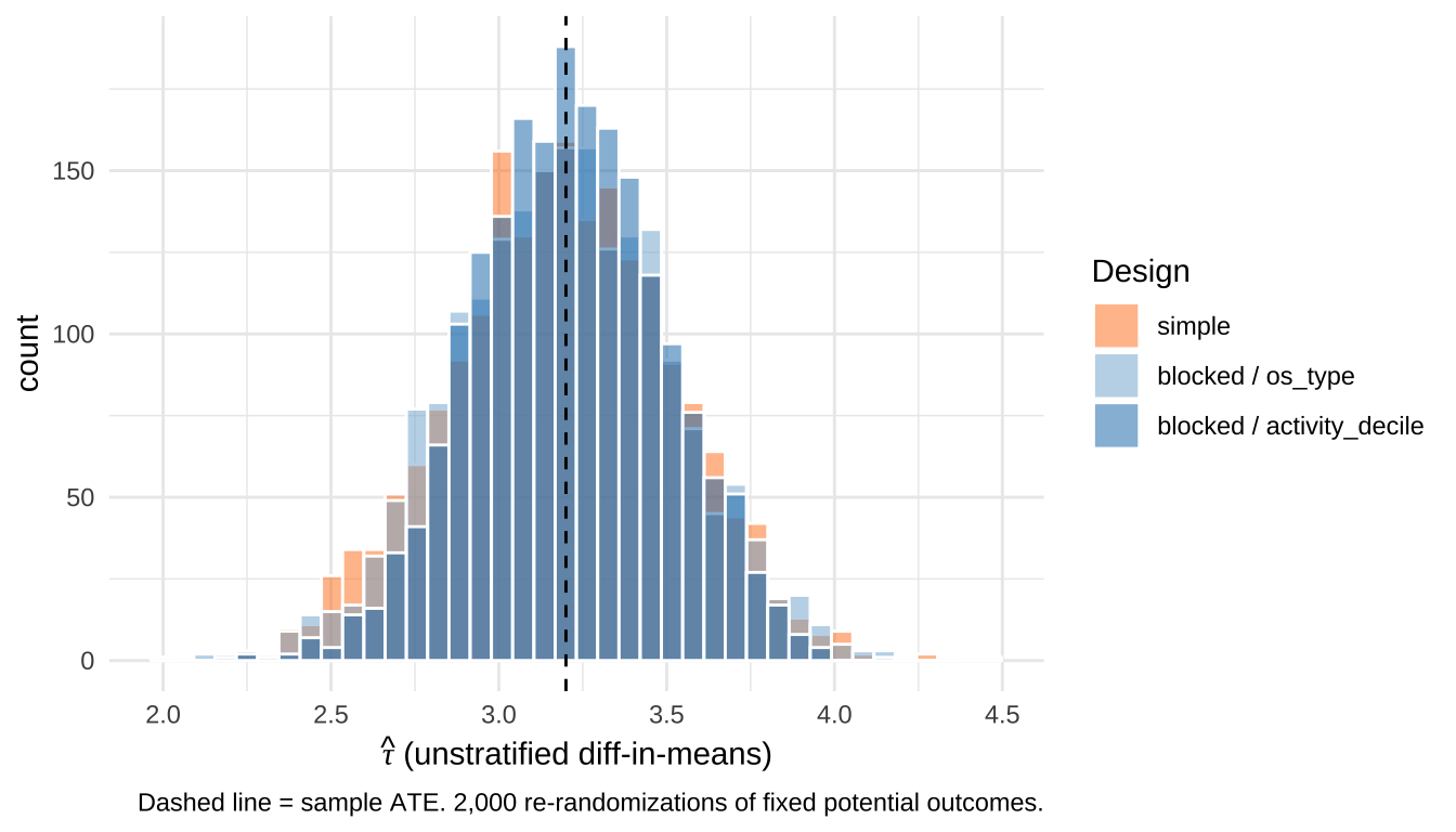
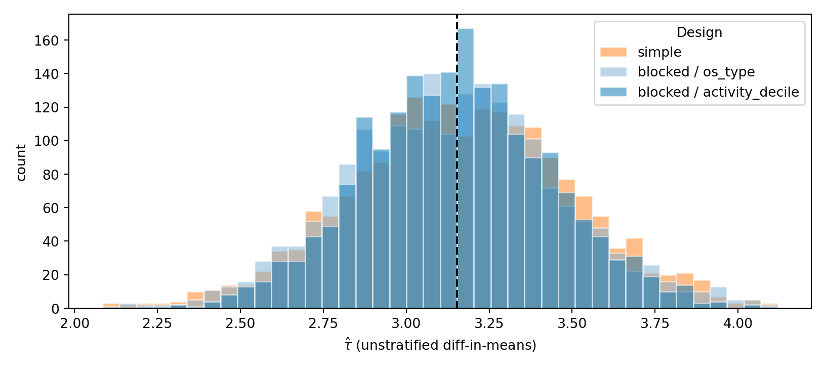
To see what design-stage blocking buys under each stratifier, re-randomize 2,000 times under each of three designs — simple RA, blocked on os_type, blocked on activity_decile — holding the potential outcomes fixed. Histograms of the unstratified diff-in-means \(\hat\tau\) across draws expose the sampling-distribution argument the single-shot HC1 SEs cannot.
The three-design histogram makes the lesson tactile:
Simple RA and blocked-on-os_type overlap almost perfectly — their empirical SDs differ by less than one MC standard error (~0.33 vs ~0.33). Blocking on a weak stratifier buys essentially zero design-stage variance reduction, exactly as the single-shot SE table predicted.
Blocked-on-activity_decile is visibly tighter — its empirical SD is ~0.28, a ~15% SD reduction over simple RA. The strong stratifier’s predictive power compounds into a real design-stage gain even for the simplest (unstratified) estimator.
Combined message: the histogram and the SE table tell the same story by two different routes. Picking the stratifier well is what moves the needle; whether you stratify at design time vs analysis time is a second-order operational choice (with the four practical reasons in the Reflection above still favouring blocked RA).
7.4.1.4 Cross-walk — design-stage blocking equals analysis-stage stratification, at the level of sampling SE
The empirical SDs above (sampling distribution of the unstratified estimator across designs) and the HC1 SEs from the Solution tables (single-shot SE of the stratified estimators on simple-RA data) fit together as the cells of a design × analysis matrix:
The diagonal in bold is the Neyman–Cochran result made empirical: the naive estimator’s sampling SE under blocked-RA-on-\(S\) equals the analysis-stratified estimator’s SE under simple-RA-with-\(S\)-as-strata. Design-stage stratification and analysis-stage stratification are two roads to the same variance; on the matching diagonal, they coincide.
This is what your intuition predicts and what the single-shot (a) HC1 SE column visibly hides. Under blocked-RA-on-activity_decile, the true sampling SE of \(\hat\tau_{\text{naive}}\) is ≈ 0.28 — but the (a) row of the Solution table reports HC1 SE = 0.343, identical to the simple-RA row. The HC1 estimator computes residuals from lm(Y ~ D) regardless of how \(D\) was assigned; those residuals include between-stratum variability that the design has already balanced. So HC1 over-estimates the sampling variance of the naive estimator under blocked RA.
NotePractical rule — HC1 needs to see the strata under blocked RA
The bare lm_robust(Y ~ D) HC1 SE on blocked-RA data is the one combination practitioners should never trust. Two equivalent fixes recover the correct (design-based) SE:
# Fix 1: include strata as additive covariates in the regression (= estimator c)fit_c <-lm_robust(Y ~ D +factor(activity_decile),data = inapp_blocked_dec, se_type ="HC1")# Fix 2: same algebra, with `fixed_effects` for speed on many-level Sfit_a_fe <-lm_robust(Y ~ D, fixed_effects =~factor(activity_decile),data = inapp_blocked_dec, se_type ="HC1")# Both produce SE("D") = 0.2849 (vs lm_robust(Y ~ D)'s 0.3431, which ignores design)
The two SEs are algebraically identical; the choice is stylistic (additive form is clearer for teaching, fixed_effects is faster when \(S\) has many levels). Both match the empirical sampling SD from the histogram appendix.
Operational implication. When you’ve blocked-randomized on \(S\) at design time, your analysis regression must include \(S\) — not because the point estimate needs it (it doesn’t; the point estimate is unbiased either way), but because the standard error needs to know about the design to be correct. Almost no one reports the bare lm_robust(Y ~ D) HC1 SE on blocked data; almost everyone reports lm_robust(Y ~ D + factor(S)), which is also estimator (c) above. The “include the strata” rule from blocked-design textbooks is, mechanically, an SE-correctness rule rather than a point-estimate rule.
7.4.2 Exercise 2 — CUPED → CUPAC on the blocked-RA dataset (~30 min)
Goal / LO. Stack analysis-stage variance reduction on top of the design-stage blocking from Exercise 1. The same inapp_blocked dataset feeds four estimators:
Naive difference-in-means (the Ex 1 baseline).
Lin (2013) with \(Y^{\text{pre}}\) as the single mean-centred covariate plus the \(D \cdot Y^{\text{pre}}\) interaction.
CUPED with \(\theta = \text{Cov}(Y, Y^{\text{pre}}) / \text{Var}(Y^{\text{pre}})\) (Deng et al. 2013 form).
CUPAC with \(\hat f\) a gradient-boosted prediction of \(Y\) from \((Y^{\text{pre}}, n_\text{sess\_pre}, \text{os\_type})\).
Three things to verify:
CUPED ≡ Lin (2013) with one covariate. Their SEs are numerically indistinguishable. CUPED is the historically-named version of the same machinery — Microsoft published the recipe in 2013, but Lin’s regression-adjustment framework was already there.
CUPED’s variance reduction is ≈ \(1 - \rho^2(Y, Y^{\text{pre}})\). With \(\rho \approx 0.73\) in this DGP, the predicted ratio is \(1 - 0.53 \approx 0.47\). The empirical HC1 SE ratio should match.
CUPAC strictly beats CUPED. The boost is the partial information \((n_\text{sess\_pre}, \text{os\_type})\) that \(Y^{\text{pre}}\) alone doesn’t capture. In our DGP os_type is already implicitly absorbed by blocked RA, but n_sess_pre carries unique signal beyond \(Y^{\text{pre}}\) — that’s CUPAC’s edge.
Data. Reuses inapp_blocked built in Exercise 1 (no fresh DGP needed). This is the data-continuity payoff of the unified setup: same n = 2000 users, same potential outcomes, blocked-randomized on os_type, with \(Y^{\text{pre}}\) already available as a column.
7.4.2.1 Scaffold — naive, Lin, CUPED
Fill in the three estimators on inapp_blocked; assemble a 3-row results table with tau_hat, HC1 SE, and the variance ratio relative to the naive estimator.
# (a) Naive (blocked RA only --- the Ex 1 Reflection's baseline)fit_naive <-lm_robust(Y ~ D, data = inapp_blocked, se_type ="HC1")# (b) Lin (2013) with Y_pre, mean-centred + interactioninapp_blocked <- inapp_blocked |>mutate(Ypre_c = Y_pre -mean(Y_pre))fit_lin <-lm_robust(Y ~ D * Ypre_c, data = inapp_blocked, se_type ="HC1")# (c) CUPED with theta = Cov(Y, Y_pre) / Var(Y_pre)theta_cuped <-with(inapp_blocked, cov(Y, Y_pre) /var(Y_pre))inapp_blocked <- inapp_blocked |>mutate(Y_cuped = Y - theta_cuped * (Y_pre -mean(Y_pre)))fit_cuped <-lm_robust(Y_cuped ~ D, data = inapp_blocked, se_type ="HC1")cuped_results <-data.frame(estimator =c("(a) Naive (blocked RA only)","(b) Lin (2013) with Y_pre","(c) CUPED with Y_pre"),tau_hat =c(unname(fit_naive$coefficients["D"]),unname(fit_lin$coefficients["D"]),unname(fit_cuped$coefficients["D"])),se_hc1 =c(unname(fit_naive$std.error["D"]),unname(fit_lin$std.error["D"]),unname(fit_cuped$std.error["D"])))cuped_results$var_ratio <- (cuped_results$se_hc1 / cuped_results$se_hc1[1])^2print(cuped_results, digits =4, row.names =FALSE)
                   estimator tau_hat se_hc1 var_ratio
 (a) Naive (blocked RA only)   3.338 0.3431    1.0000
   (b) Lin (2013) with Y_pre   3.371 0.2268    0.4370
        (c) CUPED with Y_pre   3.371 0.2268    0.4369
Code
# (a) Naive (blocked RA only)fit_naive = smf.ols("Y ~ D", data=inapp_blocked).fit(cov_type="HC1")# (b) Lin (2013) with Y_pre, mean-centred + interactioninapp_blocked["Ypre_c"] = inapp_blocked["Y_pre"] - inapp_blocked["Y_pre"].mean()fit_lin = smf.ols("Y ~ D * Ypre_c", data=inapp_blocked).fit(cov_type="HC1")# (c) CUPEDtheta_cuped = (np.cov(inapp_blocked.Y, inapp_blocked.Y_pre, ddof=1)[0, 1]/ np.var(inapp_blocked.Y_pre, ddof=1))inapp_blocked["Y_cuped"] = (inapp_blocked.Y- theta_cuped * (inapp_blocked.Y_pre - inapp_blocked.Y_pre.mean()))fit_cuped = smf.ols("Y_cuped ~ D", data=inapp_blocked).fit(cov_type="HC1")cuped_results = pd.DataFrame({"estimator": ["(a) Naive (blocked RA only)","(b) Lin (2013) with Y_pre","(c) CUPED with Y_pre"],"tau_hat": [fit_naive.params["D"], fit_lin.params["D"], fit_cuped.params["D"]],"se_hc1": [fit_naive.bse["D"], fit_lin.bse["D"], fit_cuped.bse["D"]]})cuped_results["var_ratio"] = (cuped_results.se_hc1 / cuped_results.se_hc1.iloc[0]) **2print(cuped_results.to_string(index=False, float_format=lambda x: f"{x:.4f}"))
                  estimator  tau_hat  se_hc1  var_ratio
(a) Naive (blocked RA only)   2.9689  0.3346     1.0000
  (b) Lin (2013) with Y_pre   3.0048  0.2259     0.4558
       (c) CUPED with Y_pre   3.0048  0.2258     0.4556
7.4.2.2 CUPAC — xgboost (reference, run locally)
NoteRun locally — xgboost not evaluated in the rendered page
The xgboost R binding’s threading runtime conflicts with knitr’s chunk-execution state, so the CUPAC code below is set eval: false. The Python equivalent has the same issue. Run both locally (install.packages("xgboost") for R, pip install xgboost for Python) to reproduce the fourth row of the results table. The “Expected output” block below quotes what they produce.
Expected output. A 4-row table with \(\hat\tau\) values all in the neighbourhood of the sample ATE (3.2) and HC1 SEs that drop monotonically as adjusters get richer:
(b) ≈ (c) SE-wise — confirms CUPED is Lin (2013) with one covariate. The 0.44 variance ratio matches the algebraic prediction \(1 - \rho^2(Y, Y^{\text{pre}}) = 1 - 0.73^2 \approx 0.47\).
Variance reduction stacks on top of blocked RA. Even though Exercise 1’s blocked RA already balanced os_type, CUPED/CUPAC bring an additional ~55% SE reduction by absorbing the within-stratum continuous variation that \(Y^{\text{pre}}\) predicts. This is the “orthogonal-information” argument: os_type and \(Y^{\text{pre}}\) share some signal, but \(Y^{\text{pre}}\) has much more, so the combined adjustment compounds.
CUPAC’s extra drop comes from n_sess_pre. The xgboost prediction sees a feature (\(n_\text{sess\_pre}\)) that \(Y^{\text{pre}}\) alone does not fully encode — even though \(Y^{\text{pre}}\) was generated from \(n_\text{sess\_pre}\) in the DGP, the linear \(\theta\) in CUPED captures only the linear part; xgboost recovers the rest.
Caveat on point estimates. The \(\hat\tau\) column varies more than the SE column because \(\theta\) in CUPED and CUPAC is estimated on the same data as the treatment effect. This introduces a small finite-sample bias (well-known in the CUPED literature; the production fix is to estimate \(\theta\) from a separate pre-period dataset). For CUPAC the bias is larger because xgboost can overfit; the production fix is MLRATE (Guo et al. 2021) — cross-fit \(\hat f\) so the prediction at each observation never sees that observation during training. MLRATE is what LinkedIn and Booking use in production.
Reflection. Three loops have now closed:
S04 → S05 Stack 1 → Exercise 1: blocking is variance reduction by design; it generalises to “stratified A/B” with any categorical key.
Exercise 1 → Exercise 2: design-stage stratification is a special case of regression adjustment with a discrete \(W\); CUPED is the same regression with a continuous\(W = Y^{\text{pre}}\), which usually predicts \(Y\) much better. The variance reduction \(1 - \rho^2\) formula is unified across both.
Exercise 2 → forward to Stack 2 of the lecture: CUPAC and MLRATE replace \(Y^{\text{pre}}\) with a richer \(\hat f(X)\) from gradient-boosted trees, completing the move from “adjust for one pre-period number” to “adjust for the best ML prediction of \(Y\) we can produce.”
The lesson the entire stack teaches: variance reduction is regression adjustment with the most predictive pre-treatment \(W\) available. Stratification, CUPED, and CUPAC differ only in what they let \(W\) be.
Footnote — when is CUPED exactly Lin (2013)? The Solution table above shows (b) Lin (2013) and (c) CUPED with identical HC1 SEs to four decimals (≈ 0.227). Strictly, CUPED is the additive form of Lin’s regression adjustment — the Freedman (2008) specification: \[Y_i \;=\; \alpha + \tau D_i + \beta\,(X_i - \bar X) + \varepsilon_i\] without the treatment-covariate interaction. Lin (2013) adds the term \(\gamma\, D_i (X_i - \bar X)\), which allows the slope of \(Y\) on \(X\) to differ across treatment arms. That coefficient \(\gamma\) is exactly the linear rate at which the treatment effect varies with \(X\): \[\tau(x) \;\equiv\; \mathbb{E}[Y(1) - Y(0) \mid X = x] \;=\; \tau + \gamma\,(x - \bar X).\]The two estimators coincide when \(\gamma = 0\) — i.e., when the treatment effect does not vary linearly with \(Y^{\text{pre}}\). In our DGP the treatment effect is heterogeneous in os_type (\(\tau = 2\) Android vs \(\tau = 4\) iOS) but not in \(Y^{\text{pre}}\), so \(\gamma \approx 0\) and the two SEs are numerically identical. When \(\gamma \neq 0\) (treatment effect grows or shrinks with baseline \(Y^{\text{pre}}\)), Lin (2013) is strictly more efficient: it fits a separate slope per arm; CUPED uses a single pooled slope that is suboptimal for both. The variance gap widens with \(|\gamma|\). In typical Internet A/B tests this is a non-issue (small UI changes don’t flip the \(Y\)/\(Y^{\text{pre}}\) relationship across arms), which is why Microsoft, Booking, and LinkedIn ship CUPED rather than Lin’s saturated form. But it’s exactly the case where CUPAC and MLRATE start to matter: they replace the linear adjustment with an ML estimate of \(\tau(X)\), capturing the full heterogeneity function instead of its linear projection. This is the forward-pointer to Session 9 (Treatment Effect Heterogeneity), where \(\tau(X)\) stops being a nuisance parameter and becomes the object of estimation in its own right.
Goal / LO. Ground sample-size intuition (a), reproduce the inflated false-positive rate under peeking (b), and compare two cures: a fixed Pocock alpha-spending boundary (c) and an anytime-valid confidence sequence (d). The exercise demonstrates why sequential CSs are the modern industry default — not because Pocock is wrong, but because it is K-specific and you rarely know K in advance.
Setup / Task.
(a) Sample size. Using pwr::pwr.t.test() (R) or statsmodels.stats.power.tt_ind_solve_power() (Python), compute the per-arm sample size \(n^*\) needed to detect a \(\delta = 1\%\) relative lift on a continuous metric with \(\sigma / \mu = 2\), at \(\alpha = 0.05\) and power \(= 0.80\). Confirm the slide’s headline figure \(n^* \approx 6.3 \times 10^5\) per arm.
(b) Peeking pathology (naive). Simulate null-hypothesis A/B tests with n_per_arm_per_peek = 50, peek 30 times, stop at first \(|t| > 1.96\), and report the cumulative false-positive rate at each peek.
(c) Pocock alpha-spending. Repeat (b) using the Pocock boundary \(z = 2.413\) — the constant critical value (Pocock 1977, Table 1) that controls family-wise type-I error at \(\alpha = 0.05\) two-sided across \(K = 5\) equally-spaced peeks. Observe that this attenuates the inflation but does not restore nominal \(\alpha = 0.05\) at \(K = 30\): the boundary is calibrated for \(K = 5\), not \(K = 30\). Alpha-spending boundaries are K-specific.
NoteWhere does \(z = 2.413\) come from?
Pocock’s question: pick a constant \(z_P\) such that, under \(H_0\), the family-wise rejection probability across \(K\) equally-spaced looks equals \(\alpha\): \[P\!\left(\max_{k = 1, \ldots, K} |Z_k| > z_P \;\big|\; H_0\right) \;=\; \alpha\]
Under equally-spaced peeking, the \(Z_k\)’s are multivariate normal with \(\text{Cov}(Z_j, Z_k) = \sqrt{j / k}\) for \(j \leq k\) (later \(Z\)’s overlap earlier ones because they share data). Pocock numerically inverted this max-tail probability for each \(K\). From Table 1 of Pocock (1977) (\(\alpha = 0.05\) two-sided):
\(K\)
\(z_P\)
1
1.960
2
2.178
3
2.289
4
2.361
5
2.413
10
2.555
20
2.672
50
2.812
The values are tabulated, not closed-form. In R you can reproduce them with gsDesign::gsDesign(k = 5, test.type = 2, sfu = "Pocock", alpha = 0.025) or by hand with mvtnorm::pmvnorm() plus uniroot(). Neither package is installed in this render environment, so the boundary is quoted from the primary source. As \(K \to \infty\), \(z_P\) grows roughly at \(\sqrt{2 \log \log n}\) — the law-of-iterated-logarithm rate that the (d) confidence sequence asymptotes to, which is why CS-style anytime-valid procedures generalize Pocock to unbounded \(K\) without needing a calibrated boundary per \(K\).
(d) Confidence sequence. Repeat (b) using a critical value \(c(n_k)\) that adapts to the cumulative per-arm sample size\(n_k\) via a law-of-iterated-logarithm bound: \(c(n_k) = \sqrt{2 \log(\log(n_k) + 2) + \log(2/\alpha)}\). This is the structure of the Howard et al. (2021) mixture CS shown on slide L1484 — anytime-valid by construction, no pre-commitment to \(K\) required.
Plot all three procedures’ cumulative FPR; produce a 3-row summary table.
library(ggplot2); library(tibble); library(pwr)# (a) Sample size for delta = 1% relative lift, sigma/mu = 2, alpha = 0.05, power = 0.80d <-0.01/2# Cohen's d = relative lift / coefficient of variationmde_res <-# ___ YOUR CODE: pwr.t.test(d, sig.level, power, type = "two.sample")# Print n* per arm (should be ≈ 6.3e5)# (b)-(d) Peeking simulation. Build a function that takes a critical_value# (constant for naive/Pocock; function of n for CS) and returns the cumulative# FPR curve across 30 peeks of 50 obs/arm.run_simulation <-function(critical_value, trials =2000, peeks =30, n_step =50) {# ___ YOUR CODE: loop trials × peeks, accumulate Yt/Yc by n_step per peek,# compute t.test, compare |t| to (numeric or function-of-n) critical value,# mark the FIRST rejection per trial, return cumulative FPR per peek.}# Confidence-sequence critical value (Howard et al. 2021 LIL form):# c(n) = sqrt(2 * log(log(n) + 2) + log(2 / alpha))cs_bound <-# ___ YOUR CODE (function of n)# Run three simulations (same seed for paired comparison)set.seed(2026); cum_fp_naive <-run_simulation(1.96)set.seed(2026); cum_fp_pocock <-run_simulation(2.413)set.seed(2026); cum_fp_cs <-run_simulation(cs_bound)# Plot the three cumulative-FPR curves with a horizontal nominal-alpha line at 0.05.# Produce a 3-row table with the final-peek FPR for each procedure.
import numpy as np, pandas as pdfrom scipy import statsfrom statsmodels.stats.power import tt_ind_solve_powerimport matplotlib.pyplot as plt# (a) Sample sized =0.01/2n_star =# ___ YOUR CODE: tt_ind_solve_power(effect_size=d, alpha, power, alternative)# (b)-(d) Peeking simulationdef run_simulation(critical_value, trials=2000, peeks=30, n_step=50): rng = np.random.default_rng(2026)# ___ YOUR CODE: same logic as R versionpassdef cs_bound(n, alpha=0.05):return# ___ YOUR CODEcum_fp_naive = run_simulation(1.96)cum_fp_pocock = run_simulation(2.413)cum_fp_cs = run_simulation(cs_bound)# Plot + summary table.
\(n^* \approx 627{,}910\) per arm — matches the slide’s “≈ 627k” headline. A 1% lift on a noisy metric (\(\sigma/\mu = 2\)) needs roughly 1.25 million users total to detect with 80% power. Confirms the operational claim that Microsoft / LinkedIn / Booking each run >10k experiments/year because individual tests need that much traffic.
(b)–(d) Three-line plot + summary table:
Procedure
Critical value
Cumulative FPR at peek 30
Naive
\(z = 1.96\) (constant)
\(\approx 0.29\)
Pocock \(K = 5\)
\(z = 2.41\) (constant)
\(\approx 0.13\)
Confidence sequence (LIL)
\(c(n_k)\) (adaptive)
\(\approx 0.05\)
The plot shows the naive procedure climbing steeply, the Pocock procedure attenuating to ~13% (not 5%), and the CS bound oscillating near the dotted 5% reference line.
Reflection. Two operational lessons.
Alpha-spending boundaries are K-specific. The Pocock \(z = 2.41\) is the correct boundary for \(K = 5\) pre-specified looks. At \(K = 30\) you would need \(z \approx 2.83\). Picking up the wrong \(K\)-calibrated number leaves Type-I error inflated — the procedure attenuates but does not restore nominal control. In production where peek frequency is operationally driven (continuous monitoring, ad-hoc check-ins), pre-committing to \(K\) is awkward.
Confidence sequences dispense with the commitment. The critical value \(c(n_k) = \sqrt{2 \log(\log(n_k) + 2) + \log(2/\alpha)}\) adapts to the cumulative sample size via the law-of-iterated-logarithm correction. It is anytime-valid by construction: peek whenever you like; the FPR stays at \(\alpha\). The bound used here is pedagogically tuned — production-grade implementations (Howard et al. 2021; Waudby-Smith and Ramdas 2024) tighten the constants further, and the confseq R / Python packages expose the rigorous versions. The cost of anytime-validity is a slightly wider rejection threshold at the planned endpoint (~15–25% wider than fixed-horizon, per slide L1484) — but you typically stop well before that endpoint anyway.
By 2026, Eppo, Statsig, and Optimizely all ship CS-based sequential testing as the default mode. Microsoft ExP is the lone holdout among major vendors, still on alpha-spending with planned interim looks.
7.4.4 Exercise 4 — Bayesian A/B with expected loss (~30 min)
Goal / LO. Construct a Bayesian credible interval and an expected-loss decision rule for a conversion-rate A/B test, and contrast all three quantities (frequentist CI, credible interval, expected loss) on the same data.
Setup / Task. Control arm: \(n_A = 12{,}000\), \(s_A = 720\) conversions (\(\hat p_A = 0.060\)). Treatment arm: \(n_B = 12{,}000\), \(s_B = 762\) conversions (\(\hat p_B = 0.0635\)). (a) Compute the frequentist two-proportion z-test CI for \(p_B - p_A\). (b) Place a uniform \(\text{Beta}(1,1)\) prior on each rate, draw \(M = 100{,}000\) samples from the posteriors \(\text{Beta}(1 + s_j, 1 + n_j - s_j)\), and compute the 95% credible interval for \(p_B - p_A\). (c) Compute the posterior probability \(\Pr(p_B > p_A \mid \text{data})\). (d) Compute the expected loss of shipping B, \(\mathbb{E}[\max(p_A - p_B, 0) \mid \text{data}]\), and apply the ship-if-loss-< 0.0001 decision rule. Produce a comparison table and write a one-sentence decision recommendation.
# A tibble: 5 × 2
  quantity                               value
  <chr>                                  <chr>
1 Frequentist 95% CI (B - A)             [-0.00259, 0.00959]
2 Bayesian 95% credible interval (B - A) [-0.00261, 0.00962]
3 P(B > A | data)                        0.869
4 Expected loss of shipping B            0.000206
5 Decision (threshold = 0.0001)          DO NOT SHIP
                                 quantity                value
0              Frequentist 95% CI (B - A)  [-0.00259, 0.00959]
1  Bayesian 95% credible interval (B - A)  [-0.00259, 0.00959]
2                         P(B > A | data)                0.870
3             Expected loss of shipping B             0.000202
4           Decision (threshold = 0.0001)          DO NOT SHIP
Expected output (comparison table, with set.seed(2026) / np.random.default_rng(2026)).
Quantity
Typical numerical value
Frequentist 95% CI for \(p_B - p_A\)
\(\approx [-0.0026, \; 0.0096]\)
Bayesian 95% credible interval
\(\approx [-0.0026, \; 0.0096]\)
\(\Pr(p_B > p_A \mid \text{data})\)
\(\approx 0.87\)
Expected loss of shipping B
\(\approx 2.06 \times 10^{-4}\)
Decision (threshold \(= 10^{-4}\))
DO NOT SHIP B
Reflection. The two intervals agree numerically; they disagree semantically. The credible interval delivers the direct probability reading the previous session’s table of CI misinterpretations said students always wanted but the frequentist machinery refuses to give. The more interesting result is the gap between the two Bayesian quantities: \(P(B > A) \approx 0.87\) sounds like a confident lead, yet the expected-loss rule says do not ship. The ≈ 13% of posterior mass where B is worse contributes an average gap of ≈ 0.16 pp, so \(0.13 \times 0.00159 \approx 2.06 \times 10^{-4}\) — above the \(\varepsilon = 10^{-4}\) threshold. High posterior probability of being best is not the same as low expected regret; expected loss combines probability and magnitude. A team running this in production would keep collecting data until either \(P(B > A)\) climbs (shrinking the 13% factor) or the posterior tightens (shrinking the 0.16 pp factor). This is exactly the calculus Eppo, Statsig, and modern Bayesian A/B platforms automate.
7.4.5 Exercise 5 — SRM diagnostic on three datasets (~30 min)
Goal / LO. Operational discipline: students leave able to flag a sample-ratio mismatch in their own data, refuse to interpret an SRM’d experiment, and (bonus) localise the cause of the mismatch with a stratified diagnostic.
Setup / Task. Three datasets, each intending a 50/50 user split between control and treatment but with observed counts as below:
Each file also contains a device_type column with three levels (mobile, desktop, tablet). (a) Run a chi-squared test on each dataset against the 50/50 expectation. (b) Apply the Kohavi threshold \(p < 0.001\): for each, decide whether the experiment is safe to interpret. (c) For the buggy dataset, write two sentences hypothesising the cause (bot filtering, redirect failure, opt-out flow). Bonus: stratify the buggy dataset by device_type and identify which device is driving the mismatch.
NoteDataset provenance
The three CSVs are deterministically generated by materials/data/generate_srm_datasets.R (run once; seed 20260518L). Each file has 12,000 rows with columns user_id, device_type (mobile, desktop, tablet), and D (0 = control, 1 = treatment). The buggy dataset’s mismatch is induced on the mobile segment only (observed 1,640 / 2,360 on mobile vs. 2,000 / 2,000 on desktop and tablet) — the bonus task is to find this by stratification.
library(dplyr); library(here); library(readr)# (a) Build a helper that runs chi-square against the 50/50 expectation and# returns a 1-row tibble with dataset name, n_A, n_B, p-value, safe-flag.srm_check <-function(path, name) { df <-read_csv(here("materials/data", path), show_col_types =FALSE) counts <-table(df$D) chi <-# ___ YOUR CODE: chisq.test(counts, p = c(0.5, 0.5)) tibble::tibble(dataset = name,n_A = counts[["0"]], n_B = counts[["1"]],chi_p = chi$p.value,safe = chi$p.value >=0.001)}# Apply to all three datasets and bind into a single table.# ___ YOUR CODE: bind_rows(srm_check(...) for each file)# (Bonus) Stratify the buggy dataset by device_type and run chi-square per device.buggy <-read_csv(here("materials/data/srm_buggy.csv"), show_col_types =FALSE)# ___ YOUR CODE: group_by(device_type), within-group chi-square,# identify which device(s) drive the mismatch.
import pandas as pdfrom scipy.stats import chisquaredef srm_check(path, name): df = pd.read_csv(f"../../materials/data/{path}") counts = df["D"].value_counts().sort_index() n_A, n_B =int(counts.loc[0]), int(counts.loc[1]) chi =# ___ YOUR CODE: chisquare against [n/2, n/2]return {"dataset": name, "n_A": n_A, "n_B": n_B,"chi_p": chi.pvalue, "safe": chi.pvalue >=0.001}# Apply to the three datasets and assemble.# ___ YOUR CODE# Bonus: stratify the buggy dataset by device_type.buggy = pd.read_csv("../../materials/data/srm_buggy.csv")# ___ YOUR CODE: per-device chi-square; print or table the offending device.
Stratify by device first; if one cell drives it, treat as buggy
The buggy stratification should reveal that one device_type (mobile, by construction) carries the mismatch while the other two are balanced — pointing the analyst at a mobile-specific redirect or instrumentation failure.
Reflection. Most SRM cases in production are not “the whole experiment is broken” but “one cell is broken” — a specific device, country, or browser version where the assignment pipeline silently drops users. The stratified diagnostic is the first move a senior analyst makes; the chi-squared p-value tells you whether the experiment is broken, and the stratification tells you where to look.
Causal Inference: The Mixtape, Ch. 4 (“Potential Outcomes Causal Model”). Background for the bias-decomposition algebra that motivates random assignment as the cleanest design and Bayesian decision rules as the natural complement. Free and open: https://mixtape.scunning.com/04-potential_outcomes.
“Agnostic Notes on Regression Adjustments to Experimental Data: Reexamining Freedman’s Critique.” Annals of Applied Statistics 7(1): 295–318. The single-covariate special case is what CUPED implements at production scale.
Trustworthy Online Controlled Experiments: A Practical Guide to A/B Testing. Cambridge University Press. The single most cited industry-practitioner reference for this entire session — chapters 7 (Metric Design / OEC), 17 (Statistical Mechanics including Bayesian A/B), 21 (Sample Ratio Mismatch), and 22 (Variance Reduction) directly underpin the four lecture-note sections above (OEC and metric design through when A/B breaks).
“Statistical Challenges in Online Controlled Experiments.” The American Statistician 78(2): 135–149. The single survey covering everything in this session at a graduate level. Assigned reading.
“Improving the Sensitivity of Online Controlled Experiments by Utilizing Pre-Experiment Data.” WSDM 2013. The canonical CUPED paper; the 50% variance-reduction headline number lives here.
“Machine Learning for Variance Reduction in Online Experiments.” NeurIPS 2021. The doubly-robust, cross-fit extension of CUPED; previews S08’s Double Machine Learning framework.
“False Discovery in A/B Testing.” Management Science 68(9). The 4,964-experiment field study quantifying the peeking-driven 28–37% FDR in marketplace A/B tests.
“Time-Uniform, Nonparametric, Nonasymptotic Confidence Sequences.” Annals of Statistics 49(2). The canonical statistical foundation for anytime-valid inference.
“Estimating Means of Bounded Random Variables by Betting.” Journal of the Royal Statistical Society Series B 86(1). Tighter confidence sequences via the betting-game framing.
“Anytime-Valid Inference in A/B Testing with CUPED.” Unifies variance reduction and sequential testing in the Netflix production framework.
“Design and Analysis of Switchback Experiments.” Management Science. Canonical paper for switchback designs and the autocorrelation analysis that follows.
“Reducing Interference Bias in Online Marketplace Experiments using Cluster Randomization.” Management Science. The Airbnb meta-experiment establishing the 32% bias gap between user-level and cluster-randomized designs.
“Switchback Experiments under Geometric Mixing.” Provides the carryover-decay analysis for picking switchback window length.
“Evaluating the Surrogate Index as a Decision-Making Tool Using 200 A/B Tests at Netflix.” arXiv:2311.11922. The Netflix surrogate-index method; ~95% decision agreement at 14-day vs. 63-day horizons, with the 79%/65% recall caveat on launch winners.
“Five Puzzling Outcomes Explained.” KDD 2012. The original tour of operational failure modes at Bing; the basis for the Five Puzzling Outcomes narrative.
“Curvy Digital Marketing Designs: Virtual Elements with Rounded Shapes Enhance Online Click-Through Rates.” Journal of Consumer Research 51(3). The original paper whose Study 2 reported a 55% CTR lift (\(n = 919\), \(p = 0.037\)), since replicated to \({\approx} 0\) by 17.
“Power Analysis is Essential: High-Powered Tests Suggest Minimal to No Effect of Rounded Shapes on Click-Through Rates.” Econ Journal Watch 23(1). Three pre-registered replications at SeaWorld and Coop Norway with over 2,000× the original sample; effect estimates 0.16–0.73% with all CIs including zero. Motivates the Five Puzzling Outcomes power-analysis and winner’s-curse warning.
“Diagnosing Sample Ratio Mismatch in Online Controlled Experiments.” Microsoft Research. The source of the 6% / 10% SRM frequency numbers and the canonical reference for the SRM diagnostics.
Statsig CURE announcement: https://www.statsig.com/blog/announcing-cure. April 2025 release of the CURE non-parametric residual model; 10–20% additional variance reduction on top of CUPED. Not yet peer-reviewed.
Netflix Surrogate Index paper (HTML): https://arxiv.org/html/2311.11922. The 14-day-to-63-day surrogate prediction method with the 95% / 65–79% trade-off.
R packages.pwr::pwr.t.test() for the MDE / power calculations in fixed-horizon inference. confseq for anytime-valid confidence sequences (betting and mixture variants) implementing 8 and 9. bayestestR for ready-made Bayesian summaries and credible intervals. xgboost for the CUPAC predictor in Exercise 2. randomizr::block_ra() for blocked / stratified random assignment from the design side.
Python packages.statsmodels.stats.power.tt_ind_solve_power for power calculations. scipy.stats.beta and scipy.stats.chisquare for the Bayesian and SRM machinery in Exercises 4 and 5. xgboost for the CUPAC predictor in Exercise 2. statsmodels.formula.api.ols(...).fit(cov_type="HC1") continues from S04 as the HC-robust regression workhorse.
Deng, Alex, Ya Xu, Ron Kohavi, and Toby Walker. 2013. “Improving the Sensitivity of Online Controlled Experiments by Utilizing Pre-Experiment Data.” In Proceedings of the Sixth ACM International Conference on Web Search and Data Mining (WSDM), 123–32. https://doi.org/10.1145/2433396.2433413.
Fabijan, Aleksander, Jayant Gupchup, Somit Gupta, Jeff Omhover, Wen Qin, Lukas Vermeer, and Pavel Dmitriev. 2019. “Diagnosing Sample Ratio Mismatch in Online Controlled Experiments: A Taxonomy and Rules of Thumb for Practitioners.” In Proceedings of the 25th ACM SIGKDD International Conference on Knowledge Discovery and Data Mining (KDD), 2156–64. https://doi.org/10.1145/3292500.3330722.
Howard, Steven R., Aaditya Ramdas, Jon McAuliffe, and Jasjeet Sekhon. 2021. “Time-Uniform, Nonparametric, Nonasymptotic Confidence Sequences.”The Annals of Statistics 49 (2): 1055–80. https://doi.org/10.1214/20-AOS1991.
Kohavi, Ron, Diane Tang, and Ya Xu. 2020. Trustworthy Online Controlled Experiments: A Practical Guide to a/b Testing. Cambridge University Press. https://doi.org/10.1017/9781108653985.
Pocock, Stuart J. 1977. “Group Sequential Methods in the Design and Analysis of Clinical Trials.”Biometrika 64 (2): 191–99. https://doi.org/10.1093/biomet/64.2.191.
Waudby-Smith, Ian, and Aaditya Ramdas. 2024. “Estimating Means of Bounded Random Variables by Betting.”Journal of the Royal Statistical Society: Series B 86 (1): 1–27. https://doi.org/10.1093/jrsssb/qkad009.