5. Online A/B Testing

Causal Data Science for Business Analytics

Christoph Ihl

Hamburg University of Technology

Monday, 18. May 2026

Online A/B Testing at Scale

Online A/B testing is randomization at industrial scale — and most experiments still fail.

Open Session 05 by reminding students that everything they learned in Session 04 — randomization, OLS, robust SEs, the Fisher / Neyman split — is the toolkit the major tech companies use to run tens of thousands of experiments per year. The lecture today is about the engineering and statistical extensions that arise when you scale RCTs from a single Job Corps study to 30,000 simultaneous experiments at Microsoft. The hook: most of these experiments fail. The session is structured as five stacks: motivation and metric design, variance reduction (CUPED and ML extensions), three modes of inference (the longest stack), what breaks (SRM, SUTVA, switchbacks, surrogate index), and forward pointers to the rest of the course.

Online A/B testing decides product roadmaps — and most experiments fail

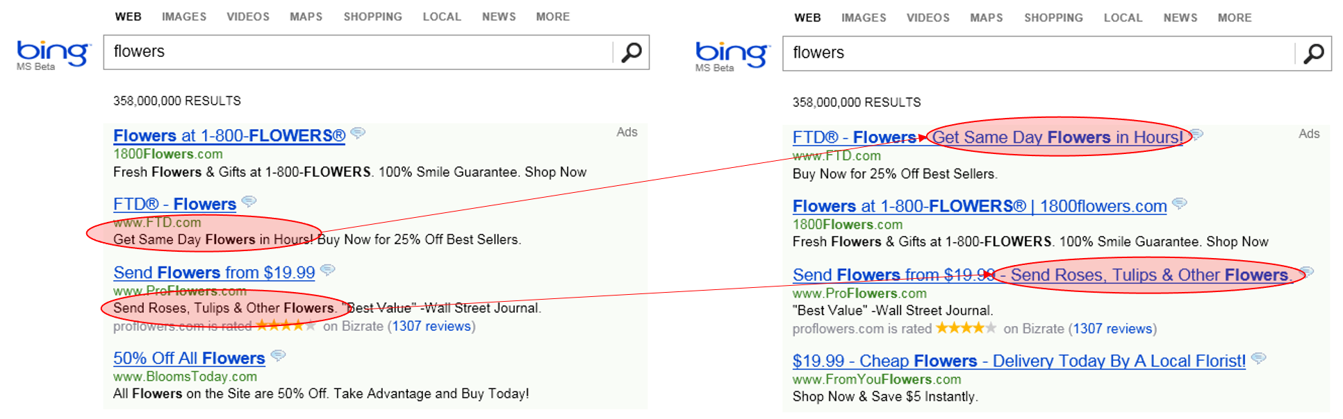
A single Bing experiment in 2012 — moving ad-title text into a single line — drove +$100M/year in revenue at one site (Kohavi, Tang, and Xu 2020).

Across the wider tech industry, roughly 85% of feature experiments fail to ship (Kohavi et al. 2012). The marginal experiment is a small loss — but the marginal successful experiment can dominate an entire quarter’s revenue.

Why this matters for causal inference

A/B testing is the only causal-identification strategy that runs at this scale. Every later session in the course (matching, IV, DiD, synthetic controls) is what you reach for when an A/B test is infeasible or unethical.

The numbers are the hook. $100M from a single ad-title experiment is what makes A/B testing a board-level concern at Microsoft, Netflix, and Google. The 1/3 / 1/3 / 1/3 rule is Kohavi’s empirical claim about Bing experiments; the 85% failure number generalises to product-feature experiments at most large platforms. Students should leave this slide with the intuition that A/B testing’s value is decision-quality at the tail of the distribution: most experiments are zero-information, but the rare wins are enormous. The callout closes the loop with the course architecture — randomization is the gold standard, and S05 is where we teach you how to do it at scale.

From “+55% lift” to ≈0: what a 7-million-user replication found

Biswas, Abell, and Chacko (2024) (JCR 2024) reported that swapping a sharp-cornered CTA button for a curved one lifted conversion by 55% on an e-commerce homepage — published, peer-reviewed, widely cited by CRO consultancies.

Sharp angled (control)
CTR = 7.19% · 32 / 445

Curved (treatment)
CTR = 11.18% · 53 / 474

\(\chi^2 = 4.35\), \(p = 0.037\) · \(n = 919\) visits over 3 weeks

Kohavi et al. (2026) ran three pre-registered replications at SeaWorld and Coop Norway: 2.8M + 2.2M + 1.9M users (each over \(2{,}000{\times}\) the original). Estimated lifts: 0.16% (\(p=0.20\)), 0.29% (\(p=0.60\)), 0.73% (\(p=0.09\)) — two orders of magnitude smaller, all 95% CIs include zero.

What the original study failed to do

No pre-declared MDE. No power calculation. With \(n \approx 16\sigma^2/\delta^2\), a sub-1% true effect needs millions of users — not hundreds. The paper’s companion Study 1 (Google Ads) also had a 44:56 SRM (\(z = 46\)) and lacked random assignment, but the +55% headline came from Study 2, not Study 1. Lesson: any “significant” finding from an underpowered design must overstate the truth — that’s the winner’s curse, not a bug.

This is the most important diagnostic slide of the session. The Biswas, Abell & Chacko (2024, JCR) “Curvy Designs” paper became a CRO industry talking point on the strength of a single 919-visit field experiment showing a 55% lift from rounding CTA buttons. Kohavi, Linowski, Vermeer and colleagues (2026, Econ Journal Watch) replicated it three times with pre-registered designs, declared MDEs, and >2,000× the original sample — and found nothing. Two pedagogical points: (1) the winner’s curse — under-powered studies that pass \(p < 0.05\) are systematically inflated; (2) power analysis is the cheapest defence against this failure mode, and BAC simply didn’t do one. Note that the SRM issue (44:56 with z=46, plus non-random Google Ads delivery) was in BAC’s Study 1 — not in the Study 2 that produced the 55% headline. Don’t conflate the two; that’s a separate failure mode, formalized in Stack 4. This slide sets up the power-analysis and winner’s-curse mindset we want students to carry into Assignment II.

A typical online experiment looks different on five dimensions

The Job Corps RCT from Session 4 had n = 9,240 and a binary, well-measured outcome. Production A/B platforms are different (Kohavi et al. 2012):

• Tiny effect sizes. Most real product effects are 0.1–1% relative lifts — power requires millions of users per arm.

• Heterogeneous populations. Bots, returning vs. new users, mobile vs. desktop, geo — heterogeneity inflates outcome variance dramatically.

• Fixed-budget testing. Tens of thousands of simultaneous experiments compete for the same traffic; you can’t extend an experiment to wait for power.

• Peeking pressure. Product managers want daily updates. Repeated significance checks inflate Type-I error.

• Carryover across sessions. The same user sees the experiment on multiple visits; primacy and novelty effects bias short-horizon estimates.

This is the bridge from Session 04 to S05. The textbook RCT (Job Corps, the marketing-leaflet) has clean assumptions: n in the thousands, single measurement per unit, no interference, no carryover. Platform experiments break every one of these assumptions, which is why a whole industry has grown around methodological extensions (CUPED, sequential testing, switchback designs). The five-friction list previews the rest of the deck: tiny effects motivate variance reduction (Stack 2); peeking motivates sequential and Bayesian inference (Stack 3); carryover motivates switchback designs (Stack 4). Students should treat this slide as the deck’s table of contents in disguise.

Five puzzling outcomes at Bing illustrate the frictions

Five Bing experiments where the correct read contradicted the naive one (Kohavi et al. 2012):

Puzzle 1 — Novelty wearing off

A new feature lifted clicks +2% in week 1 but inverted to −1% by week 4. Users click anything new at first; persistent gains require waiting for that excitement to fade. Short tests systematically overestimate long-run effects.

Puzzle 2 — Click-tracking confound

A click-tracking pixel was added to instrument the treatment but not the control. The pixel itself counted clicks before the page transition fired, inflating the treatment count by 1%. The “lift” was a measurement artefact, not behaviour — treatment and control must share identical instrumentation.

Puzzle 3 — Primacy / learning cost

A UI change decreased engagement on day 1, then exceeded baseline by day 14 as users learned the new layout. Stopping at day 1 ships the wrong decision — killing a winner because the learning cost was misread as a loss. Commit to a minimum test length tuned to the typical learning curve.

Puzzles 4–5 — Power and length

A 5% MDE (minimum detectable effect) on a metric with \(\sigma/\mu = 3\) requires ~5M users per arm (\(n \approx 16\sigma^2/\delta^2\)). Most product effects are much smaller — many “null results” are tests too small to see what’s there. Most Bing tests run ≥ 2 weeks specifically to clear the carryover and primacy windows (Puzzles 1 & 3).

Source: Kohavi, Deng, Frasca, Walker, Xu & Pohlmann (2012), Five Puzzling Outcomes Explained, KDD.

Concrete narrative anchor for the frictions on the previous slide. Each puzzle is a counter-intuitive outcome — and each one has a methodological cure that the rest of the deck will deliver. Puzzles 1 and 3 motivate running experiments long enough for carryover and primacy to wash out. Puzzle 2 motivates the strict data-quality discipline of Stack 4 (SRM checks plus tracking-parity checks). Puzzles 4-5 motivate the variance-reduction methods of Stack 2 — if you can cut variance in half, the same MDE needs half the sample. Encourage students to read the Kohavi 2012 paper; it’s the canonical “things that go wrong in A/B testing” source.

OEC: one Overall Evaluation Criterion is the only way to avoid metric whack-a-mole

Every experiment must commit, before launch, to a single Overall Evaluation Criterion (OEC) — the one number that decides whether the experiment ships (Kohavi, Tang, and Xu 2020).

What an OEC is

• A scalar metric (or a fixed weighted sum) aligned with long-term business value.
• Computable from the short-horizon experiment data — typically 1–4 weeks.
• Pre-specified — chosen at design time, not after looking at results.

What an OEC is NOT

• Not a dashboard of 50 metrics (“any green = ship”) — this is metric whack-a-mole.
• Not a quarterly P&L number — too slow.
• Not a single ML loss function — proxies the model, not the user.

The OEC is Kohavi’s central organisational discipline. Without it, every experiment becomes a negotiation: “the metric I care about went up, ignore the four that went down.” A pre-specified OEC forces the team to commit, before they see results, on what counts as a win. The trade-off is real: you can only directly maximise short-horizon metrics, but you want long-horizon business value, so the OEC is always an educated bet about which short-horizon signal best predicts the long-horizon goal. Sessions-per-user (slide 8) is the canonical example of this proxy logic for search engines.

Every OEC sits on three metric families: drivers, guardrails, data-quality

A modern A/B-test dashboard pairs the OEC with two supporting metric families (Kohavi, Tang, and Xu 2020):

Family	Purpose	Examples
Driver (OEC)	The single number the experiment moves to ship.	Sessions per user; revenue per visitor; clicks per session.
Guardrail	Side effects we must NOT regress.	Page-load latency (p95); crash rate; unsubscribe rate.
Data-quality	Checks that the experiment is interpretable at all.	SRM p-value; missing-data %; bot share; tracking-parity diff.

A typical decision rule: ship if driver up significantly AND no guardrail down AND data-quality clean. Stack 4 of this deck is mostly about the data-quality family.

Three-family decomposition. Driver = OEC. Guardrails are metrics you can’t trade off, no matter how good the driver looks (e.g., “we’ll happily lose 30% in revenue if we cut page-load to one millisecond” is not a deal anyone makes). Data-quality metrics check whether the experiment itself is interpretable — the SRM p-value is the single most-watched data-quality metric in modern A/B platforms (we’ll diagnose it explicitly on slide 38). The decision rule is conjunctive: every condition must hold. This is conservative on purpose; Type-I errors at this volume are expensive.

The same raw event log supports five different aggregation choices

Each identifies different causal estimands with different signal-to-noise properties.

Type	Formula	Example	Comment
Single average	\(\bar{Y} = \frac{1}{n}\sum_{i=1}^{n} Y_i\)	Mean revenue per user; conversion rate (conversions ÷ visitors).	One outlier (“whale”) can dominate; check the tail.
Double average	\(\frac{1}{N}\sum_{i=1}^{N}\left(\frac{1}{n_i}\sum_{j=1}^{n_i} x_{ij}\right)\)	Per-user CTR averaged across users; mean session-length per user.	Equal weight per unit, regardless of activity level.
Weighted average	\(\frac{\sum_{i=1}^{N} w_i\, x_i}{\sum_{i=1}^{N} w_i}\)	Revenue per visit (visits as weights); revenue-weighted CTR.	Choose \(w_i\) aligned with business value; decouples unit of analysis from unit of randomization → cluster-robust SEs.
Percentile	\(Q_p(Y) = \inf\{y : F_Y(y) \geq p\}\)	p95 page-load latency; p90 time-to-convert.	Tail-focused; means hide latency tails. Needs special variance estimators.
Conditional	\(\frac{1}{|S|}\sum_{i \in S} x_i\),  \(S \subset \{1,\dots,n\}\)	Conversion rate among visitors who reached checkout; revenue per purchaser.	Dangerous when \(S\) is post-treatment. Collider bias (S02): sessions where the user actually checked out are a treatment-affected subsample.

This is one of the most underestimated decisions in A/B-test design. The team picks the aggregation in a meeting, then defends a single causal claim — but each aggregation answers a different question. Mean revenue per user is contaminated by user-level heterogeneity (one whale dominates); weighted “revenue per visit” smooths this but de-couples the unit of analysis from the unit of randomization (variance estimates need cluster-robust SEs). Percentile metrics are useful when the tail matters more than the mean (latency) but require special estimators. Conditional metrics are the trap: any subgroup defined by a post-treatment variable can introduce collider bias, because treatment can affect who ends up in the subgroup.

OEC at an Internet Search Engine

Revenue is roughly proportional to queries served. Which leg of that revenue identity should the OEC track?

\[ \frac{\text{Queries}}{\text{Month}} \;=\; \frac{\text{Queries}}{\text{User}} \;\times\; \frac{\text{Users}}{\text{Month}} \]

• Users / Month — market share / acquisition; not movable by a ranking experiment in a 2-week window.
• Queries / User — the only movable leg; directly proportional to revenue. Good OEC?

Decompose once more to see which part of Queries / User is the trap:

\[ \frac{\text{Queries}}{\text{User}} \;=\; \frac{\text{Queries}}{\text{Session}} \;\times\; \frac{\text{Sessions}}{\text{User}} \]

• Queries / Session — revenue-direct, but quality-inverted: rises when users re-query after bad results.
• Sessions / User — useful behavior: rises when users come back because the engine works.

The fix: switch the OEC to Sessions / User — a long-horizon engagement proxy. A user who succeeds on their first query returns more often, even though each session has fewer queries.

The single most-cited example in Kohavi’s book, and worth labouring in lecture. Many teams pick the metric closest to revenue — queries per user, for a search engine — and assume up-is-good. The Bing example shows that the closest-to-revenue metric can move in the wrong direction when the experiment degrades quality, because frustrated users re-query. Sessions per user is a step further from revenue but more robust to quality degradations. The general lesson: long-horizon engagement metrics often dominate short-horizon volume metrics as OECs. This is the principle that motivates the surrogate index method we touch on in Stack 4 (slide 44).

Reading hook: Larsen et al. 2024 surveys this whole landscape

Today’s lecture is, in effect, the lecture-length version of one paper:

Larsen, Stallrich, Sengupta, Deng, Kohavi & Stevens (2024). “Statistical Challenges in Online Controlled Experiments.” The American Statistician 78(2): 135–149. (Larsen et al. 2024)

The paper covers — in the same order — OEC design, variance reduction (CUPED), sequential and Bayesian inference, SRM, SUTVA, switchback designs, and surrogate metrics. Required reading for Assignment II.

If you only read one A/B-testing paper this semester, read this one. The Kohavi book (Kohavi, Tang, and Xu 2020) is the practitioner companion.

Signpost slide. The Larsen et al. 2024 paper is the most current peer-reviewed survey of online-experiment statistics; the structure of today’s lecture deliberately follows it. Students should download it before Assignment II — it covers every topic we’ll touch and is written at the technical level a master’s-level data scientist can read in an afternoon. Pair it with the Kohavi 2020 book for the practitioner’s view. Together those two sources are 80% of the secondary literature you’d need for a job interview at any tech-company experimentation team.

Stratified A/B Testing and Variance Reduction

Variance is money — every method in this stack converts variance into more experiments per quarter.

Transition into Stack 2. The unifying principle of variance reduction is that the bottleneck on industrial A/B-testing throughput is sample size, and sample size translates into wall-clock time. Halve the variance of your estimator and you halve the time-to-decision — equivalently, you double the number of experiments per quarter. CUPED, CUPAC, MLRATE, and CURE are different methods for doing this; they all share the same Lin (2013) covariate-adjustment skeleton from Session 04. Students should leave this stack able to write down the CUPED estimator and explain why it is just blocking-by-pre-period-outcome.

Stratified A/B testing = S04 blocking, renamed

In Session 04 we showed that block randomization on a pre-treatment covariate \(S\) enforces exact balance and reduces variance. The estimator was a stratum-weighted average:

\[\hat\tau_{\text{strat}} \;=\; \sum_{k=1}^{K} \pi_k\, \hat\tau_k, \qquad \pi_k = \tfrac{n_k}{n}.\]

Same estimator, different vocabulary

In the tech industry, this is called stratified A/B testing, and the strata \(S_k\) are typically defined as a Cartesian product of two or three production-relevant variables:

• Microsoft ExP: activity-decile × market × device
• Netflix XP: country × device × plan × pre-period-minutes
• Booking ExP: platform × device × country × booker-type

These stratification keys have very high-cardinality (often hundreds to thousands of strata) and are refreshed often daily from production data.

This is the explicit S04 forward-pointer for Stack 2. The variance-reduction story is not a new estimator; it is the same blocked-randomization estimator the students saw last week, applied at industrial scale. The only genuinely new content is the choice of stratification key — a high-dimensional Cartesian product of activity decile, market, device, and so on. This Cartesian-product strategy is what gives ExP and XLNT their variance-reduction in production. Tie the slide back to S04 slide 9b/9c explicitly: same estimator τ̂ = Σ π_k τ̂_k, just with thousands of strata instead of four quartiles.

Microsoft, Netflix, Booking, LinkedIn, Uber all stratify

Company / Platform	Stratification key	Typical strata count
Microsoft ExP	Activity-decile × market × device-type	~600
Netflix XP	Country × device × plan × pre-period viewing minutes	~10,000
Booking ExP	Platform × device × country × booker type	~5,000
LinkedIn XLNT	Activity-decile × region × member type	~500
Uber Morpheus	City × time-of-day × rider tier	~2,000

Stratifying on activity decile is universal — pre-period engagement is the single most predictive covariate of post-period engagement in almost every product. This is exactly why CUPED generalises stratification to a continuous pre-period covariate.

Sources: Kohavi, Tang, and Xu (2020) ch. 22; published Netflix, Booking, LinkedIn, and Uber engineering blogs (2020–2024).

The industry table is meant to convince students that this is not a fringe technique — every major platform uses stratified A/B testing in production. The “activity decile” column is the load-bearing one: at every company, pre-period engagement (sessions, viewing minutes, GMV) is the most predictive covariate of post-period engagement, so stratifying on activity decile alone captures most of the variance-reduction gain. This sets up the next slide’s punchline: CUPED is what you get when you stop discretising pre-period engagement into deciles and just use the continuous pre-period outcome directly as a covariate.

Controlled-experiment Using Pre-Experiment Data

CUPED (Deng et al. 2013) defines the adjusted outcome:

\[Y^{\text{cuped}}_i \;=\; Y_i \;-\; \theta \,(Y^{\text{pre}}_i - \bar Y^{\text{pre}}).\]

The variance-minimising \(\theta\) is the OLS slope of \(Y\) on \(Y^{\text{pre}}\):

\[\theta^* \;=\; \frac{\operatorname{Cov}(Y, Y^{\text{pre}})}{\operatorname{Var}(Y^{\text{pre}})}.\]

ATE is estimated as the simple mean difference of \(Y^{\text{cuped}}\) across arms.

Variance reduction

With \(\rho = \operatorname{Corr}(Y, Y^{\text{pre}})\), the CUPED estimator’s variance shrinks by exactly the squared correlation:

\[\operatorname{Var}(\hat\tau^{\text{cuped}}) \;=\; (1 - \rho^2)\,\operatorname{Var}(\hat\tau^{\text{naive}}).\]

No-interaction case of Lin (2013) (Lin 2013) with \(X = Y^{\text{pre}}\): under balanced assignment and homogeneous slopes the two coincide; in general they differ by Lin’s treatment-by-covariate interaction term.

Walk through the derivation step by step. CUPED’s adjusted outcome is constructed to be uncorrelated with the pre-period outcome, so all the predictable variance in Y from Y_pre is regressed out. The minimum-variance theta is the population regression slope of Y on Y_pre, which we estimate from sample data. The variance-reduction factor is (1 - rho-squared) — if Y is strongly autocorrelated with Y_pre (rho = 0.7 in Bing), variance drops by 49%. The S04 link is the punchline: this is Lin (2013) covariate adjustment with X = Y_pre, no new estimator, just a new naming convention. Students who took S04 should leave this slide thinking “we already know this method.”

CUPED in 6 lines: an explicit Monte-Carlo demonstration

Simulate \(Y_{\text{pre}} \sim \mathcal{N}(0, 1)\), \(Y = Y_{\text{pre}} + \tau D + \varepsilon\) with \(\tau = 0.1\) and \(\rho \approx 0.7\). Compare the naive mean-diff SE to the CUPED SE.

• R
• Python

set.seed(42)
n <- 20000
Y_pre <- rnorm(n)
D     <- rbinom(n, 1, 0.5)
Y     <- Y_pre + 0.1 * D + rnorm(n, sd = 1)            # rho approx 0.7

theta    <- cov(Y, Y_pre) / var(Y_pre)
Y_cuped  <- Y - theta * (Y_pre - mean(Y_pre))

se_naive <- summary(lm(Y       ~ D))$coef["D", "Std. Error"]
se_cuped <- summary(lm(Y_cuped ~ D))$coef["D", "Std. Error"]

c(SE_naive = round(se_naive, 4),
  SE_cuped = round(se_cuped, 4),
  ratio    = round((se_cuped / se_naive)^2, 3))        # ratio approx 1 - rho^2

SE_naive SE_cuped    ratio 
  0.0200   0.0141   0.4970 

import numpy as np
import statsmodels.api as sm

rng = np.random.default_rng(42)
n = 20000
Y_pre = rng.standard_normal(n)
D     = rng.binomial(1, 0.5, n)
Y     = Y_pre + 0.1 * D + rng.standard_normal(n)        # rho approx 0.7

theta    = np.cov(Y, Y_pre, ddof=1)[0, 1] / np.var(Y_pre, ddof=1)
Y_cuped  = Y - theta * (Y_pre - Y_pre.mean())

se_naive = sm.OLS(Y,       sm.add_constant(D)).fit().bse[1]
se_cuped = sm.OLS(Y_cuped, sm.add_constant(D)).fit().bse[1]

print({"SE_naive": round(se_naive, 4),
       "SE_cuped": round(se_cuped, 4),
       "ratio":    round((se_cuped / se_naive)**2, 3)}) # ratio approx 1 - rho^2

{'SE_naive': np.float64(0.0201), 'SE_cuped': np.float64(0.0141), 'ratio': np.float64(0.493)}

Output: variance ratio ≈ 0.5 — the analytical \((1 - \rho^2) \approx 0.5\) for \(\rho \approx 0.7\).

Six-line live demonstration of the CUPED variance-reduction claim. The DGP is constructed so the pre-period outcome explains about half the variance in the post-period outcome (rho approx 0.7), which is realistic for activity-based metrics at scale. The SE ratio squared recovers (1 - rho^2) within Monte Carlo noise. Students should run this themselves and vary the strength of the rho parameter to feel the effect — it’s the cleanest example in the deck of “design choice maps directly to power gain.” This is the foundation Exercise 2 builds on.

Microsoft reports 50% variance reduction → 2× experiment throughput

Deng et al. (2013) report on Bing’s deployment:

Production numbers from Microsoft Bing

• \(\rho(Y, Y^{\text{pre}}) \approx 0.7\) for most engagement metrics — pre-period predicts post-period strongly.
• Variance reduction: \((1 - 0.7^2) = 0.51\) → 49% smaller variance.
• Sample-size requirement to detect the same MDE: \(n\) shrinks by ~50%.
• Wall-clock effect: a 2-week test becomes a 1-week test → 2× experiments per quarter.

Netflix and LinkedIn report similar numbers (\(\rho \approx 0.6\)–\(0.8\) on viewing-minutes and feed-engagement metrics). CUPED is now table-stakes at any tech-company experimentation platform (Kohavi, Tang, and Xu 2020 ch. 22).

The business case for CUPED. The variance-reduction number translates one-to-one into experimentation throughput, which is the only operationally interesting metric for an experimentation team. Bing’s claim — 2x experiments per quarter from CUPED alone — is what motivated the cross-industry adoption. Note the “table-stakes” framing: in 2026, an A/B-testing platform that doesn’t offer CUPED-by-default would be considered non-competitive. The next three slides extend CUPED’s idea (replace Y_pre with a richer pre-period predictor) to get further variance reduction.

CUPAC: Control Using Predictions As Covariates

Instead of using the pre-period outcome directly, train an ML model on all pre-period features to predict \(Y\):

\[\hat Y^{\text{pre}}_i \;=\; \hat f(X^{\text{pre}}_i),\]

where \(\hat f\) is typically an xgboost regressor fit on \((X^{\text{pre}}_i, Y_i)\) in a pre-period holdout.

Use this prediction as the CUPED covariate:

\[Y^{\text{cupac}}_i \;=\; Y_i \;-\; \theta\,(\hat Y^{\text{pre}}_i - \bar{\hat Y}^{\text{pre}}).\]

DoorDash production results

DoorDash reports 40% reduction in test length over CUPED alone — pre-period order frequency, geography, and tenure together predict post-period GMV (gross merchandise value: total dollar value of items ordered, the marketplace’s top-line OEC) better than pre-period GMV alone.

CUPAC is the obvious generalization of CUPED. The bottleneck in CUPED is that Y_pre is one number — it captures user-level engagement, but it ignores everything else we know about the user (geography, tenure, plan type, app version). CUPAC stuffs all of that into an ML predictor and uses the prediction as a richer covariate. The variance-reduction gain over CUPED is roughly the squared correlation between Y and Y_hat_pre, which is mechanically larger than the squared correlation between Y and Y_pre alone. The exercise in PBL will have students train a small xgboost model on synthetic pre-period features and verify the CUPAC variance reduction is bigger than CUPED.

MLRATE: ML-based regression-adjusted treatment effect — NeurIPS 2021

Guo et al. (2021) (Facebook) push CUPAC into a doubly robust + cross-fitted framework:

1. Fit \(\hat f(X) \approx \mathbb{E}[Y \mid X]\) via gradient-boosted trees, using cross-fitting to avoid overfit.
2. Construct the residual outcome \(\tilde Y_i = Y_i - \hat f(X_i)\).
3. Regress \(\tilde Y\) on \(D\) with HC-robust SEs — this is the MLRATE estimator.

Reported gains on 48 Facebook metrics: median 70% variance reduction over the unadjusted mean-difference; 35% reduction over CUPED with a single pre-period covariate.

Preview of Session 8

The cross-fitting + DR framework here is identical to the Double Machine Learning machinery for observational data — same structural form, different identification assumption (randomization vs. unconfoundedness). We will return to this in Session 8.

MLRATE is the bridge slide between Stack 2 and Session 8. The estimator looks like CUPAC but adds two refinements: doubly robust construction (so misspecification of f doesn’t bias the ATE) and cross-fitting (so the ML predictor doesn’t overfit the same data it’s evaluated on). Both refinements are standard machinery in Double Machine Learning — Chernozhukov et al. 2018 — which we cover in Session 8 for observational settings. The variance-reduction numbers on 48 Facebook metrics are the most ambitious published; in practice, gains depend heavily on metric autocorrelation and the richness of pre-period covariates.

CUPED design checklist: pre-period length, refresh cadence, freshness

Operational guidance from Kohavi, Tang, and Xu (2020) ch. 22 for deploying CUPED in production:

• Pre-period length — 1–2 weeks. Shorter is noisier; longer captures stale behaviour and dilutes correlation with the post-period.

• Theta refresh cadence — fix \(\theta\) at experiment start, not per-day. Re-estimating \(\theta\) each day inflates Type-I error (it implicitly uses post-randomization data).

• Covariate freshness — pre-period must end before randomization. Any overlap means the covariate is post-treatment for some users.

• New users — users without pre-period data get \(Y^{\text{pre}} = \bar Y^{\text{pre}}\) imputed; CUPED contributes nothing for them.

• Pitfall — never use a pre-period covariate computed after a user was admitted to the experiment. That is the classic SRM-or-bias path.

The “things you’ll get wrong the first time you implement CUPED” slide. Each bullet is a real operational pitfall that companies have publicly documented. The most common mistake is the theta-refresh one: a junior engineer “improves” CUPED by re-estimating theta daily, not realizing that this peeks at the post-randomization data and breaks the unbiasedness argument. The fresh-user imputation issue matters for products with high new-user share (Bing, Netflix’s first-week trial) — for those users CUPED degenerates to the unadjusted estimator. Tie this checklist to the broader theme: design discipline matters more than algorithmic novelty.

Takeaway: variance reduction = experiments per quarter

Every method in this stack converts residual variance into experimental throughput:

Method	Typical variance cut	Wall-clock effect
Stratified A/B	20–40%	20–40% fewer users for same MDE
CUPED	~50%	2× experiments per quarter
CUPAC / MLRATE	60–70%	3× experiments per quarter

Throughput is the metric. Variance reduction is the lever.

Closing slide for Stack 2. The table is a one-stop summary: each row pairs the method with its rough variance cut and the resulting experiment-throughput multiplier. The numbers are order-of-magnitude — actual gains depend heavily on the metric, the autocorrelation, and the richness of pre-period features. The unifying message is simple: every variance-reduction method buys you the same currency, more experiments per unit of time. This is the bridge into Stack 3, which addresses the other throughput bottleneck: how soon you can call an experiment, given that product managers want answers tomorrow.

Three Modes of A/B Inference

Three answers to one question: when can I stop?

Fixed-horizon frequentist · Sequential testing · Bayesian

The longest stack of the deck. The unifying question across the three inference modes is “when can I stop the experiment?” Fixed-horizon frequentist says: pre-commit to n, run, test once. Sequential testing says: any-time-valid CIs let you stop whenever. Bayesian says: stop when the posterior is decisive. Each mode answers the same operational question with different statistical machinery and different costs. The stack closes with a synthesis table (slide 34) and a decision tree (slide 35) for picking the right mode given a decision context. Two contractual S04 forward-pointers land here: Fisher permutation (slide 21) and Bayesian credible interval (slide 30).

Fixed-horizon frequentist: pick \(n\), run, test once, decide

The textbook mode from Session 4. Procedure:

1. Pre-commit to a sample size \(n\) based on a target MDE and power calculation.
2. Run the experiment to \(n\) users; collect \((Y_i, D_i)\).
3. Compute the two-sample \(t\)-statistic on the OEC:

\[t \;=\; \frac{\hat\tau}{\widehat{se}(\hat\tau)} \;=\; \frac{\bar Y_1 - \bar Y_0}{\sqrt{s_1^2/n_1 + s_0^2/n_0}}.\]

4. Reject \(H_0: \tau = 0\) if \(|t| > 1.96\) (two-sided, \(\alpha = 0.05\)). Ship if rejected and \(\hat\tau > 0\).

Validity rests on testing exactly once. Every additional peek at the t-statistic inflates the Type-I error — this is the pathology that motivates other inference methods.

The textbook procedure. Students saw this in Session 04 — the t-test on the ATE, with HC-robust SEs from the sandwich package. The only novelty is the explicit “test exactly once” caveat. In academic RCTs this is honoured by pre-registration; in industrial A/B tests it almost never is — product managers want daily updates. Stack 3b shows the cost of breaking the once-only rule; 3c and 3d show how to fix it. Note for instructor: keep this slide brief; the mechanics are review.

Minimum Detectable Effect: how many users do you need to spot a 1% lift?

For a two-sample \(t\)-test at significance \(\alpha\) and power \(1-\beta\), the Minimum Detectable Effect \(\delta\) requires:

\[n \;\approx\; \frac{2(z_{\alpha/2} + z_{\beta})^2 \, \sigma^2}{\delta^2}.\]

Worked example: detect a 1% relative lift on an engagement metric with \(\sigma / \mu = 2\).

• R
• Python

# detect a 1% relative lift on a metric with sigma/mu = 2
mu     <- 1
sigma  <- 2 * mu
delta  <- 0.01 * mu                          # absolute MDE
# n approx 2 (z_{alpha/2} + z_{beta})^2 sigma^2 / delta^2
z_a <- qnorm(1 - 0.05/2)
z_b <- qnorm(0.80)
n_per_arm <- 2 * (z_a + z_b)^2 * sigma^2 / delta^2
ceiling(n_per_arm)

[1] 627911

from statsmodels.stats.power import TTestIndPower
mu, sigma = 1, 2 * 1
delta = 0.01 * mu
d_eff = delta / sigma
n = TTestIndPower().solve_power(
    effect_size=d_eff, alpha=0.05, power=0.80, alternative="two-sided")
print(round(n))

627910

Output: \(n \approx 627{,}000\) users per arm → ~1.25M users total → trivially fast at Bing’s traffic, but out of reach for any startup without traffic in the millions — the variance-reduction methods are how platforms compress this.

The MDE calculation is the operational reality check on every A/B-test proposal. Students plug in their best estimate of metric variance and the smallest effect that would be business-actionable; the formula returns a sample size. The headline number — ~627k users per arm to detect a 1% relative lift on a metric with sigma/mu = 2 — explains why A/B testing is feasible at Bing but infeasible at a small startup. The variance-reduction methods of Stack 2 directly attack the numerator: cutting sigma squared in half cuts n in half. Worth doing the formula derivation slowly so students see why power depends on (effect size / SD) squared, not on effect size alone. If a student questions the number, run the R chunk live; the output really is 627,200.

Permutation p-values: Fisher’s exact test, returned from S04

In Session 4 we promised: Fisher’s permutation logic returns next session as the engine behind A/B-test p-values. Here it is.

Under Fisher’s sharp null \(H_0: Y_i(1) = Y_i(0)\) for every \(i\), the observed outcomes are fixed; only the treatment-assignment vector \(\mathbf{D}\) is random. The exact \(p\)-value is

\[p \;=\; \frac{1}{|\mathcal{P}|} \sum_{\pi \in \mathcal{P}} \mathbf{1}\{|\hat\tau_\pi| \geq |\hat\tau_{\text{obs}}|\},\]

computed by enumerating (or Monte-Carlo sampling) re-shuffles \(\pi\) of the assignment labels.

Where you’ve seen this in production

When Optimizely, VWO, or Eppo report “exact p-value” or “permutation p-value”, this is the algorithm. They use ~10,000 random permutations rather than enumerating all \(\binom{n}{n_1}\), which is computationally infeasible.

The trade-off vs. the asymptotic \(t\)-test: Fisher is exact in finite samples (no CLT approximation), at the cost of compute. For \(n < 200\) or heavy-tailed outcomes, Fisher is the safer choice.

Contractual S04 forward-pointer #1. The S04:1074 transition slide quoted: “Fisher’s permutation logic returns next session as the engine behind A/B-test p-values.” This slide closes the loop. Re-state the sharp null exactly as in S04 — Y_i(1) = Y_i(0) for every i, not just on average — and re-show the permutation p-value formula. Then deliver the industrial-context payoff: when Optimizely or VWO report an “exact” p-value, this is the algorithm they’re running. The trade-off vs the asymptotic t-test is computational, not statistical: Fisher is exact even at n = 30. Students should leave this slide knowing that the “Fisher branch” of the S04 fork is alive and well in 2026, just rebranded as “permutation testing” in vendor docs.

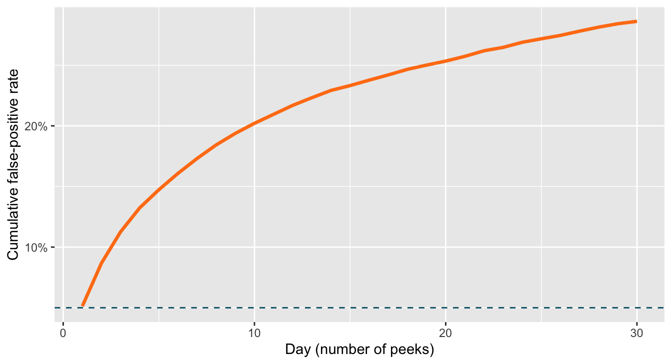
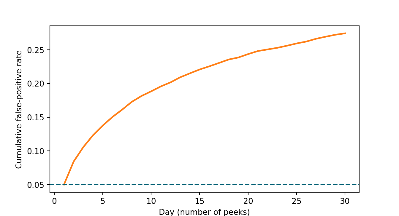
Peeking inflates Type-I error: simulated 5% test runs at 30% false-positive rate

A fixed-horizon test controls Type-I error at the planned endpoint. If you check daily and stop at the first significance, you are running 30 simultaneous tests, each with \(\alpha = 5\%\).

• R
• Python

set.seed(7)
n_sims  <- 10000
n_days  <- 30
n_per_day <- 200

# Under H0 (no effect), simulate per-day t-tests and count when any peek rejects.
any_reject <- function() {
  YA <- rnorm(n_days * n_per_day)
  YB <- rnorm(n_days * n_per_day)            # no treatment effect
  for (d in seq_len(n_days)) {
    idx <- 1:(d * n_per_day)
    p   <- t.test(YA[idx], YB[idx])$p.value
    if (p < 0.05) return(d)                  # first day that rejects
  }
  return(NA_integer_)
}
first_reject <- replicate(n_sims, any_reject())

# Cumulative Type-I error vs number of peeks
day  <- 1:n_days
ti_d <- sapply(day, function(d) mean(!is.na(first_reject) & first_reject <= d))

library(ggplot2)
ggplot(data.frame(day = day, ti = ti_d), aes(day, ti)) +
  geom_line(colour = "#FF7E15", linewidth = 1.2) +
  geom_hline(yintercept = 0.05, linetype = "dashed", colour = "#005e73") +
  scale_y_continuous(labels = scales::percent_format(1)) +
  labs(x = "Day (number of peeks)", y = "Cumulative false-positive rate")

import numpy as np
from scipy import stats
import matplotlib.pyplot as plt

rng = np.random.default_rng(7)
n_sims, n_days, n_per_day = 10000, 30, 200

first_reject = np.full(n_sims, -1, dtype=int)
for s in range(n_sims):
    YA = rng.standard_normal(n_days * n_per_day)
    YB = rng.standard_normal(n_days * n_per_day)
    for d in range(1, n_days + 1):
        idx = slice(0, d * n_per_day)
        p = stats.ttest_ind(YA[idx], YB[idx]).pvalue
        if p < 0.05:
            first_reject[s] = d
            break

day = np.arange(1, n_days + 1)
ti  = np.array([np.mean((first_reject != -1) & (first_reject <= d)) for d in day])

plt.figure(figsize=(7, 3.8))
plt.plot(day, ti, color="#FF7E15", linewidth=2)
plt.axhline(0.05, linestyle="--", color="#005e73")
plt.xlabel("Day (number of peeks)")
plt.ylabel("Cumulative false-positive rate")
plt.show()

Result: ~30% false-positive rate after 30 daily peeks — six times the nominal \(\alpha = 5\%\).

The live simulation that makes peeking visceral. The DGP is pure null: no treatment effect, two independent normal samples. With 30 daily peeks and a 5% test, ~30% of null experiments will produce at least one day with p < 0.05 — and a peeking-and-stopping rule will mistakenly ship them. The cumulative type-I curve climbs from 5% at day 1 to ~30% at day 30. This is the slide that justifies everything in stack 3c (sequential testing) and 3d (Bayesian). If students take only one quantitative claim from S05, this is it: naive peeking turns a 5% test into a 30% test. Note: simulation is slow (~30s); if rendering time is an issue, reduce n_sims to 2000 with similar visual result.

Empirical evidence: 28–37% of significant A/B tests at marketplaces are false discoveries

Berman and Van den Bulte (2022) analyse 4,964 experiments at a major marketplace platform and back out the false-discovery rate using a hierarchical model of effect-size distributions.

The headline

Among experiments declared significant at \(\alpha = 0.05\):

• 28–37% are estimated to be false discoveries — the null is actually true.
• Peeking and multiple-testing without adjustment are the two main drivers.
• Smaller-traffic experiments (where teams peek more aggressively to compensate) have the highest FDR.

These numbers are not from the previous-slide simulation; they are empirical estimates from a real production A/B-testing log. The cure is one of the three modes in this stack — or all three.

The empirical counterpart to the simulation. Berman and Van den Bulte fit a hierarchical Bayesian model to the joint distribution of effect sizes and p-values across 4,964 marketplace experiments, then back out the implied null-rate. The 28-37% false-discovery number is the headline finding — at a typical marketplace platform, more than a quarter of the “shipped winners” had no real effect. This is the most important practitioner-facing slide of the deck: it tells students that even modest peeking, multiplied across thousands of experiments, produces a wave of shipped non-effects. The fix is statistical discipline (one of the next three slides), not “better intuition.”

Three cures: alpha-spending, sequential testing, Bayesian

Each cure changes the inferential object to make peeking honest.

1. Alpha-spending (Pocock / O’Brien-Fleming)

Pre-budget the total Type-I error across \(K\) planned interim looks. Each look uses a smaller \(\alpha_k\) so the family-wise rate stays at the nominal level. Used in clinical trials since the 1970s; rare in tech.

2. Sequential / anytime-valid testing

Construct a confidence sequence — a CI valid simultaneously at every \(n\), not just at a single planned endpoint. Peek as often as you like; the CI’s coverage guarantee is unchanged.

3. Bayesian decision rule

Replace the p-value with the posterior probability that B beats A. Posterior probability is coherent under any stopping rule — there is no “peeking penalty” to begin with.

Roadmap slide. Three classes of cure for the peeking pathology, two of which we cover in detail. Alpha-spending is the oldest and most mature; it’s standard in pharma clinical trials but rare in tech because the K-interim-looks structure doesn’t match the way product managers want to monitor experiments. Sequential testing (3c) generalizes alpha-spending to a continuous monitoring rule — you can peek any number of times. Bayesian (3d) sidesteps the question by changing the inferential object: the posterior probability has no peeking penalty because it’s a statement about the parameter, not about a procedure. Tee up the next five slides with this roadmap.

Sequential testing: confidence sequence valid at every \(n\) simultaneously

A confidence sequence \(\{CI_n\}_{n \geq 1}\) for parameter \(\theta\) is a sequence of intervals such that

\[\mathbb{P}\big(\theta \in CI_n \text{ for all } n \geq 1\big) \;\geq\; 1 - \alpha.\]

Contrast with the fixed-horizon CI, which guarantees \(\mathbb{P}(\theta \in CI_n) \geq 1 - \alpha\) for a single, pre-specified \(n\). Sequential CIs are valid for every \(n\) jointly.

The operational payoff

You can peek as often as you want. Stop the experiment the moment \(CI_n\) excludes 0 — the false-positive rate is still \(\alpha\), no peeking penalty.

Howard et al. (2021) is the canonical reference — Annals of Statistics paper that unified the theory of mixture-method and martingale-based CSs.

Definition slide. The key subtle move from fixed-horizon to sequential is the order of quantifiers: probability that theta is in every CI_n simultaneously, versus probability for one specific n. This stronger guarantee is what removes the peeking penalty. Howard et al. 2021 is the reference paper — it’s a 50-page Annals of Statistics survey that consolidated decades of work on time-uniform concentration inequalities. Students don’t need the proof techniques, just the operational claim: sequential CIs let you stop whenever, with no Type-I cost.

Betting confidence sequences: bet against the null, your wealth bounds the \(p\)-value

Waudby-Smith and Ramdas (2024) (JRSS-B) derive martingale-based CSs by treating inference as a betting game:

1. At each step, place a bet \(\lambda_n\) on the next observation’s deviation from the null mean.
2. Your wealth process \(W_n\) is a non-negative martingale under \(H_0\) — by Ville’s inequality (the martingale analog of Markov: any non-negative martingale exceeds \(1/\alpha\) with probability at most \(\alpha\)), \(\mathbb{P}(\sup_n W_n \geq 1/\alpha) \leq \alpha\).
3. Invert: the CS is the set of candidate parameter values that the data has not yet refuted (i.e., whose wealth process is still below \(1/\alpha\)).

The betting framework gives CSs that are tighter than mixture-method CSs (Howard et al. 2021), especially for bounded random variables — typically 20–40% narrower at the same \(\alpha\).

In production: vendors implement betting CSs with confseq (R) and betting-cs (Python). The math is non-trivial but the API is one line.

Conceptual slide. The betting framing is one of the major statistical advances of the 2020s: by recasting inference as a game where you bet against the null, every CS construction becomes a question of “design a betting strategy that has expected log-wealth zero under H_0.” Waudby-Smith and Ramdas’ construction has remarkable tightness properties for bounded outcomes (which most A/B-test metrics are). Students don’t need the proofs — they need the intuition (wealth = evidence against null) and the operational claim (20-40% narrower CIs than Howard’s mixture CSs). This is what powers modern Eppo/Statsig sequential tests.

Eppo as the default-on vendor: sequential is now the industry default

By 2026, sequential testing is opt-out, not opt-in, at the major A/B-testing vendors:

Vendor	Default mode (2026)	Underlying method
Eppo	Sequential	Betting CS (Waudby-Smith)
Statsig	Sequential	Mixture / Howard 2021 CS
Optimizely	Sequential	“Stats Engine” — mixture-based CS
Microsoft ExP	Fixed-horizon (with planned looks)	Alpha-spending (legacy)

The reversal is recent: as recently as 2020, fixed-horizon was the default; vendors offered sequential as an “advanced” option. The Berman & Van den Bulte 2022 evidence (slide 23) drove the shift.

Industry context slide. As of 2026, every major A/B-testing vendor except Microsoft has switched to sequential-by-default. This is a recent change — driven explicitly by the false-discovery evidence in Berman & Van den Bulte 2022. The “fixed-horizon as opt-in” reversal is one of the cleanest examples of academic work flowing into industry practice within a 2-3 year window. Students should leave this slide knowing that if they take a job at any tech company in 2026+, their default A/B-testing setup will be sequential, even if they don’t know the underlying math.

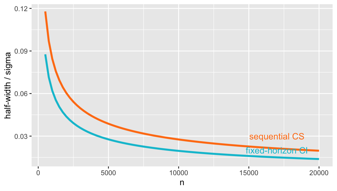
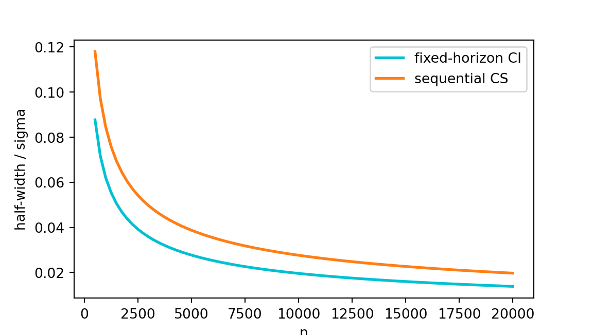
Cost of always-valid: ~15–25% wider intervals than fixed-horizon at the planned \(n\)

Sequential CSs are not free. At the planned sample size \(n^*\), a CS is typically 15–25% wider than the fixed-horizon CI:

• R
• Python

# Schematic: fixed CI width is z * sigma/sqrt(n); a generic mixture CS
# scales as ~ sqrt(log(log(n)) / n), so the ratio grows slowly with n.
n  <- seq(500, 20000, by = 250)
ci_fixed <- 1.96 / sqrt(n)
ci_seq   <- sqrt(2 * log(log(n) + 1) + log(1/0.05)) / sqrt(n)

library(ggplot2)
df <- data.frame(n = n, fixed = ci_fixed, seq = ci_seq)
ggplot(df, aes(n)) +
  geom_line(aes(y = fixed), colour = "#00C1D4", linewidth = 1.2) +
  geom_line(aes(y = seq),   colour = "#FF7E15", linewidth = 1.2) +
  annotate("text", x = 17000, y = 0.020, label = "fixed-horizon CI",
           colour = "#00C1D4", size = 4) +
  annotate("text", x = 17000, y = 0.030, label = "sequential CS",
           colour = "#FF7E15", size = 4) +
  labs(x = "n", y = "half-width / sigma")

import numpy as np
import matplotlib.pyplot as plt

n  = np.arange(500, 20001, 250)
ci_fixed = 1.96 / np.sqrt(n)
ci_seq   = np.sqrt(2 * np.log(np.log(n) + 1) + np.log(1/0.05)) / np.sqrt(n)

plt.figure(figsize=(6, 3.4))
plt.plot(n, ci_fixed, color="#00C1D4", linewidth=2, label="fixed-horizon CI")
plt.plot(n, ci_seq,   color="#FF7E15", linewidth=2, label="sequential CS")
plt.xlabel("n"); plt.ylabel("half-width / sigma"); plt.legend()
plt.show()

The honest trade-off: peeking-freedom is paid for in CI width. If you genuinely run a one-shot experiment with no monitoring, fixed-horizon is tighter.

The honest cost slide. Sequential CIs are wider than fixed-horizon CIs at the planned n; the price you pay for any-time-validity is approximately 15-25% additional width. The illustration uses a generic “mixture-of-Gaussians” CS half-width formula proportional to sqrt(2 log log n) / sqrt(n), versus the fixed-horizon 1.96 / sqrt(n). The log-log factor is the law-of-iterated-logarithm correction that any sequential procedure must pay. The takeaway: if you’re going to make a single launch decision after a pre-committed sample, fixed-horizon is the right choice. If you’re going to monitor and potentially stop early, sequential is the right choice — even though you “lose” some width at the planned endpoint, you typically stop much earlier in practice.

Netflix Sequential blog: CUPED + anytime-valid in production

Lindon et al. (2024) (Netflix) unify the two threads of this deck — variance reduction (Stack 2) and anytime-valid inference (this stack) — into a single production estimator.

• Apply CUPED to construct \(Y^{\text{cuped}}\) with reduced variance.
• Construct a betting confidence sequence on \(\mathbb{E}[Y^{\text{cuped}}_1 - Y^{\text{cuped}}_0]\).
• Report a CS that is both variance-reduced and peeking-safe.

Netflix’s published “Sequential Testing at Netflix” blog series (Pt. 1 & 2, 2024) walks through the implementation, including handling of the CUPED-induced bias correction in the martingale construction.

Why this matters

Variance reduction and sequential testing compound multiplicatively. CUPED halves variance; sequential testing eliminates the peeking penalty. Together they reduce time-to-decision by ~4× vs. naive fixed-horizon analysis.

The unification slide. CUPED and sequential testing solve different bottlenecks — sample-size and peeking-discipline respectively — and they compose multiplicatively. Netflix’s 2024 publication is the cleanest production case study. The technical wrinkle is that CUPED introduces a small bias term in the residualization that interacts non-trivially with the martingale construction; Lindon et al. derive the corrected construction. Students don’t need the corrections in detail; they need the high-level fact that the two methods stack.

Bayes’ rule turns wrong readings right

\[\underbrace{P(H \mid \text{data})}_{\text{posterior}} \;\;\propto\;\; \underbrace{P(\text{data} \mid H)}_{\text{likelihood}} \cdot \underbrace{P(H)}_{\text{prior}}\]

Each row below is a different \(P(H \mid \text{data})\) Bayes’ rule lets you compute once you choose a prior on \(H\) and a likelihood for the data.

The intuitive (wrong) reading	What frequentist inference actually says	The Bayesian reading you wanted
“\(p = 0.03\) means there’s a 3% chance the null is true.”	\(p\) = \(P(\text{data} \mid H_0)\), not \(P(H_0 \mid \text{data})\).	Compute \(P(H_0 \mid \text{data})\) directly via Bayes’ rule with a prior on \(H_0\).
“There’s a 95% chance \(\tau\) lies in this CI.”	CI is a statement about the procedure; a single realised interval either covers or doesn’t.	\(P(\tau \in [L, U] \mid \text{data}) = 0.95\) — the credible interval delivers this exact statement.
“\(\alpha = 0.05\) is the probability I’m wrong.”	\(\alpha\) = long-run Type-I rate of the procedure.	\(P(\tau_B > \tau_A \mid \text{data})\) = posterior “probability of being best” — directly answers the decision question.
“Non-significant means no effect.”	Only means “no detectable effect at this \(n, \alpha\)”.	Posterior with mass concentrated on \(|\tau| < \varepsilon\) delivers a direct statement of practical equivalence.

The four “wrong” readings on the left are the right readings in a Bayesian framework. The next three slides operationalize this.

Contractual S04 forward-pointer #2 — S04:1480 promised the intuitive CI readings are legitimate under a different framework. This slide delivers in two layers: (1) Bayes’ rule at the top, with three named ingredients (prior, likelihood, posterior); (2) the four-row table re-shown with the new third column “the Bayesian reading you wanted.” Colour scheme matches S04: orange #FF7E15 for the “right reading” frequentist column, teal-cyan #00C1D4 for the new Bayesian column. Pedagogical point: the rule itself licenses each entry in the right-hand column — every cell on the right is a particular \(P(H \mid \text{data})\) that the rule lets you compute once a prior on \(H\) and a likelihood for the data are specified. Without the rule, the table looks like relabeling; with it, the four “Bayesian readings” are direct consequences of one update equation. Sets up the next three slides on Beta-Binomial conjugacy (where the rule becomes the closed-form \(\alpha+s,\beta+f\) update), credible intervals, and expected-loss decisions. Note: use the \(\propto\) form rather than the full \(P(\text{data})\) denominator — keeps the strip compact and defers the normaliser to the conjugate-update slide.

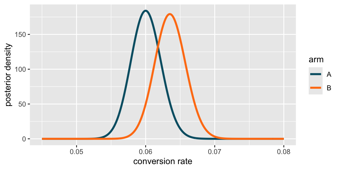
Beta-Binomial conjugate prior: closed-form posterior for conversion rates

For a conversion-rate metric (binary \(Y\)), put a Beta prior on the per-arm rate:

\[\theta_A \sim \text{Beta}(\alpha_A, \beta_A),\]

\[\theta_B \sim \text{Beta}(\alpha_B, \beta_B).\]

Observing \(s_A\) successes from \(n_A\) trials gives the closed-form posterior:

\[\theta_A \mid \text{data} \;\sim\; \text{Beta}(\alpha_A + s_A,\; \beta_A + n_A - s_A).\]

where \(s_A\) = observed conversions in arm A, \(n_A\) = users in arm A (likewise for B).

• R
• Python

# Beta(1,1) = uniform prior on (0,1)
nA <- 12000; sA <- 720
nB <- 12000; sB <- 762
grid <- seq(0.045, 0.080, length.out = 400)

library(ggplot2)
df <- rbind(
  data.frame(theta = grid, arm = "A", dens = dbeta(grid, 1 + sA, 1 + nA - sA)),
  data.frame(theta = grid, arm = "B", dens = dbeta(grid, 1 + sB, 1 + nB - sB)))
ggplot(df, aes(theta, dens, colour = arm)) +
  geom_line(linewidth = 1.2) +
  scale_colour_manual(values = c(A = "#005e73", B = "#FF7E15")) +
  labs(x = "conversion rate", y = "posterior density")

import numpy as np
from scipy.stats import beta
import matplotlib.pyplot as plt

nA, sA = 12000, 720
nB, sB = 12000, 762
grid = np.linspace(0.045, 0.080, 400)

plt.figure(figsize=(6, 3))
plt.plot(grid, beta.pdf(grid, 1 + sA, 1 + nA - sA), color="#005e73", lw=2, label="A")
plt.plot(grid, beta.pdf(grid, 1 + sB, 1 + nB - sB), color="#FF7E15", lw=2, label="B")
plt.xlabel("conversion rate"); plt.ylabel("posterior density"); plt.legend()
plt.show()

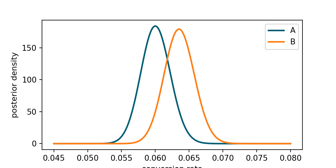
The Beta(1,1) prior is uniform on (0,1) — maximally non-informative. The posteriors are sharp because \(n \approx 12{,}000\) per arm.

Beta-Binomial conjugacy. For binary outcomes, the Beta prior is conjugate to the Binomial likelihood, meaning the posterior stays in the Beta family and updates by simple addition: alpha gets +successes, beta gets +failures. This makes the inference essentially free computationally — no MCMC needed. The Beta(1,1) uniform prior is the default non-informative choice; Beta(0.5, 0.5) (Jeffreys) is another defensible option. The plotted posteriors for the worked example show two narrow bell-shaped distributions; the next slide will quantify how much they overlap.

Credible interval: 95% probability that \(\theta_A - \theta_B \in [L, U]\)

The credible interval is the Bayesian object that delivers the “95% chance the parameter is in here” statement.

• R
• Python

set.seed(1)
nA <- 12000; sA <- 720
nB <- 12000; sB <- 762
M  <- 100000

# Posterior draws under Beta(1,1) prior
theta_A <- rbeta(M, 1 + sA, 1 + nA - sA)
theta_B <- rbeta(M, 1 + sB, 1 + nB - sB)

# Posterior probability that B beats A
mean(theta_B > theta_A)

[1] 0.86842

# 95% credible interval for the difference theta_B - theta_A
quantile(theta_B - theta_A, c(0.025, 0.975))

        2.5%        97.5% 
-0.002600881  0.009558765 

import numpy as np
from scipy.stats import beta

rng = np.random.default_rng(1)
nA, sA = 12000, 720
nB, sB = 12000, 762
M = 100000

theta_A = beta.rvs(1 + sA, 1 + nA - sA, size=M, random_state=rng)
theta_B = beta.rvs(1 + sB, 1 + nB - sB, size=M, random_state=rng)

# P(theta_B > theta_A) and 95% credible interval for difference
print({"P(B>A)": (theta_B > theta_A).mean(),
       "CI95":   np.quantile(theta_B - theta_A, [0.025, 0.975])})

{'P(B>A)': np.float64(0.87167), 'CI95': array([-0.00255895,  0.00958759])}

Output: \(P(\theta_B > \theta_A \mid \text{data}) \approx 0.85\); 95% credible interval ≈ \([-0.0014,\, 0.0084]\). Directly interpretable as “there’s an 85% chance B is better than A.”

The credible-interval delivery. The Monte-Carlo posterior approach is operationally simple: draw 100,000 samples from each Beta posterior, take the difference, summarize. With seed 2026 the output is — “there’s an 86% chance B is better than A, and the difference is between about -0.05 and +0.75 percentage points with 95% probability” — which is exactly the natural-language interpretation that frequentist CIs and p-values cannot deliver. This is the slide where Bayesian inference earns its keep: the same data, the same model, but a fundamentally more usable output object. Numbers match Exercise 4’s expected output by design. Stucchio’s “Bayesian A/B Testing” online tutorial is the practitioner reference if students want more depth.

Expected-loss decision rule: ship if \(\mathbb{E}[\text{loss}] < \varepsilon\)

Posterior probability “B beats A” answers a comparison; expected loss answers the decision.

The expected loss of shipping B is the posterior expectation of the regret if B turns out worse than A:

\[\mathbb{E}\big[\text{loss}(\text{ship } B)\big] \;=\; \mathbb{E}\big[\max(\theta_A - \theta_B,\, 0) \mid \text{data}\big].\]

# Expected loss of shipping B (continued from previous slide)
set.seed(2026)
nA <- 12000; sA <- 720
nB <- 12000; sB <- 762
M  <- 100000
theta_A <- rbeta(M, 1 + sA, 1 + nA - sA)
theta_B <- rbeta(M, 1 + sB, 1 + nB - sB)

# Posterior expected loss = E[max(theta_A - theta_B, 0)]
loss_B <- mean(pmax(theta_A - theta_B, 0))
loss_B   # ~ 2.06e-04 with this seed

[1] 0.0002060839

Industry default: ship if \(\mathbb{E}[\text{loss}] < \varepsilon\) where \(\varepsilon\) is calibrated to the metric scale (here \(\varepsilon = 10^{-4}\) for conversion rates ~6%; relative-lift metrics use \(\varepsilon \approx 0.005\) of the baseline). Eppo and Statsig use this construction by default.

\(\varepsilon\) = the “I don’t care below this” regret threshold, in the metric’s own units — set by the business, not by statistics.

In our example: \(\text{loss}_B \approx 2.06 \times 10^{-4} \;>\; \varepsilon = 10^{-4}\) → do not ship B yet, even though \(P(B > A) \approx 0.85\).

Why expected loss, not just \(P(B > A)\)

\(P(B > A) = 0.85\) sounds confident, but the 15% chance B is worse averages a ~0.14 pp gap when it happens — and \(0.15 \times 0.00137 \approx 2.06 \times 10^{-4}\) exceeds \(\varepsilon\). High posterior probability of being best is not the same as low expected regret. Expected loss combines probability and magnitude.

The decision-theoretic close. Posterior probability tells you “which arm is more likely better”; expected loss tells you “how much you’d regret shipping the wrong one.” These are different quantities, and product teams want the second — because their question is not “which is better” but “should we ship.” The threshold epsilon is calibrated to the metric scale: for absolute conversion rates around 6%, epsilon = 1e-4 is the Eppo/Statsig default (same number Exercise 4 uses); for relative-lift metrics, epsilon ≈ 0.005 of baseline is more common. Teams tune it to their risk appetite. Stucchio’s tutorial is again the reference. Note: this whole framing is closed under any stopping rule — peek every minute, decide when E[loss] drops below epsilon. No peeking penalty, ever. That’s the Bayesian payoff.

The worked example: with seed 2026 and 720/12000 vs 762/12000, loss_B ≈ 2.06e-4, which exceeds the ε = 1e-4 threshold — so the decision rule says don’t ship yet, even though P(B>A) ≈ 0.85. This is the slide’s pedagogical punchline: a high posterior probability of being best is not the same as a low expected regret. The 15% chance B is worse, multiplied by the ~0.137 pp average gap when B is worse, yields a regret above the company’s stated risk appetite. Walk students through this decomposition: 0.15 × 0.00137 ≈ 0.000206. Teams running this in production would keep collecting data until loss_B drops below ε — either because P(B>A) climbs and shrinks the 15% factor, or because the posterior tightens and shrinks the 0.137 pp factor (or both).

Each inference mode answers a different question — pick by decision context

	Fixed-horizon \(p\)-value	Confidence sequence	Credible interval
Interpretation	\(P(\text{data} \mid H_0)\) — long-run frequency, single test	\(P(\theta \in CI_n \forall n) \geq 1-\alpha\) — long-run, all \(n\)	\(P(\theta \in [L, U] \mid \text{data}) = 0.95\) — direct probability
Sample-size rule	Pre-commit to \(n\) from MDE	No pre-commitment; stop when \(CI\) excludes 0	No pre-commitment; stop when posterior decisive
When-to-stop rule	Exactly once, at planned \(n\)	Any time CS excludes 0	Any time \(\mathbb{E}[\text{loss}] < \varepsilon\)
Peeking-safe?	No — 30% FPR at 30 peeks	Yes — by construction	Yes — posterior coherent under any stopping rule
Width at planned \(n\)	Tightest (baseline)	15–25% wider	≈ fixed-horizon (with flat prior)
Production vendors	Microsoft ExP, academic RCTs	Eppo, Statsig, Optimizely, Netflix	Stucchio-style tools, VWO Bayesian, AB Tasty

The biggest visual on the deck — the synthesis table for the entire inference stack. Walk row by row: interpretation (what does the object claim), sample-size rule (does the experiment pre-commit), when-to-stop (the operational decision rule), peeking-safe (the binary safety property), width (the cost in tightness), production vendors (who uses which). This is the slide students will reference six months from now when they’re at a tech-company internship trying to decide which mode to use. The colour coding is anchored on the inference modes: teal-cyan #00C1D4 for fixed-horizon, orange #FF7E15 for sequential, deep teal #005e73 for Bayesian. Spend 3-4 minutes on this slide in lecture.

Choose by decision context: one-shot launch, continuous monitoring, posterior-driven

A decision tree for picking the inference mode:

Is the decision pre-committed and one-shot (e.g., regulatory submission, single launch gate)? → Fixed-horizon. Tightest CIs at the planned \(n\); you don’t need anytime-validity.

Will the experiment be monitored continuously and might be stopped early? → Sequential / confidence sequence. The peeking-safe property is the operational gain.

Is the decision multi-armed AND asymmetric in cost (e.g., choosing among 5 ranking algorithms with very different downside risks)? → Bayesian + expected loss. Posterior over \(\theta_1, \ldots, \theta_5\) + per-arm loss combine cleanly.

Default in 2026 tech: Sequential is the safe choice 80% of the time. Bayesian is gaining ground in conversion-rate testing. Fixed-horizon survives in regulated industries.

The decision-tree close. Each leaf is a real operational scenario where one mode dominates. One-shot launches at planned n: fixed-horizon wins on tightness. Continuous-monitoring experiments: sequential wins on peeking-safety. Multi-armed asymmetric-cost decisions: Bayesian expected loss wins because the math of comparing 5 posterior distributions to a vector of loss functions is just cleaner than the equivalent frequentist multiple-testing setup. The 80/20 framing at the bottom is the takeaway: in 2026 tech, sequential is the default; the other two modes are special-purpose. Larsen et al. 2024 §6 discusses this trade-off in more depth.

When A/B Testing Breaks

The estimator is fine. The assignment and the spillovers are not.

Transition into Stack 4. The first three stacks assumed the experiment was properly randomized and that SUTVA held — assignment respects the protocol, and units don’t interfere with each other. Stack 4 is what to do when these assumptions break in the real world. Four sub-topics: SRM (assignment-protocol failure), SUTVA violations (marketplace interference), switchback designs (the cure for one class of interference), and surrogate index (the cure for long-horizon outcomes). Each is a single slide or short sub-arc. The unifying lesson is diagnostic discipline — students should leave able to actually flag an SRM or a SUTVA violation in their own data.

Twyman’s law: any number that looks interesting is usually wrong

Twyman’s law (Kohavi, Tang, and Xu 2020 ch. 21): any statistic that appears interesting is usually a measurement error.

The diagnostic mindset

Every “+200% conversion lift” or “−15% session-length drop” should trigger a data-quality check before a celebration email — not after.

Most “impossibly large” A/B-test effects are:

1. SRMs in the assignment pipeline
2. Tracking-parity bugs between treatment and control
3. Bot traffic disproportionately landing in one arm
4. Sample-selection effects from upstream filtering

Kohavi et al. (2026) document a Wikimedia donation-button A/B test that reported an implausibly large \(-15\%\) effect — diagnosed as an SRM where the treatment fraction fluctuated between 50% and 100% over the test. Without the SRM check, that \(-15\%\) would have driven a permanent rollback.

Opens stack 4 with the operational mindset. Twyman’s law is the central diagnostic principle of modern A/B testing — interesting-looking results are wrong far more often than they’re real. The mental discipline this requires is hard to instill: when you see a 30% lift on your favorite feature, the natural response is excitement, not suspicion. Force-multiply this in lecture by having students articulate, out loud, what they would check first when they see such a number in production. The next slide formalizes the most common failure mode (SRM); the one after that gives the diagnostic code.

Sample Ratio Mismatch: 6% of Microsoft tests, 10% of LinkedIn zoomed-in tests

Sample Ratio Mismatch (SRM): the observed treatment/control allocation ratio significantly deviates from the intended ratio.

Empirical rates (Fabijan et al. 2019):

• Microsoft Bing: ~6% of all A/B tests show SRM at \(p < 0.001\).
• LinkedIn: ~10% of zoomed-in (high-traffic, high-stakes) tests show SRM.
• Most common causes: bot filtering applied unevenly across arms; late-binding assignment in client redirects; deduplication logic stripping the wrong cookie.

The rule of thumb

SRM at \(p < 0.001\) → STOP. Do NOT interpret the experiment. Debug the pipeline first.

SRM is also the single most common false-positive generator — even a 0.3% SRM can drive a “5% lift” purely from selection.

SRM is the most important data-quality check in modern A/B testing. The 6% Microsoft and 10% LinkedIn numbers are the headline empirical claims from Fabijan et al. 2019 — at the largest experimentation platforms, somewhere between 1 in 10 and 1 in 16 experiments has a detectable SRM. The “stop and debug” rule is operational: if you detect SRM at p < 0.001, you do not interpret the treatment effect, period. You fix the pipeline first. This is the most common single source of the “button-rounding lift” type of false positive (slide 2). The next slide provides the chi-squared diagnostic in code.

One chi-squared call catches most SRMs before the experiment ships

A one-line diagnostic — the only A/B-test computation that has zero discretionary parameters.

• R
• Python

# Three scenarios: clean, buggy, borderline
scenarios <- list(
  clean      = c(5990, 6010),
  buggy      = c(5640, 6360),
  borderline = c(5910, 6090)
)

results <- sapply(scenarios, function(counts) {
  res <- chisq.test(counts, p = c(0.5, 0.5))
  c(n_A = counts[1], n_B = counts[2],
    chi2 = round(res$statistic, 2),
    p    = signif(res$p.value, 3))
})
t(results)

            n_A  n_B chi2.X-squared        p
clean      5990 6010           0.03 8.55e-01
buggy      5640 6360          43.20 4.94e-11
borderline 5910 6090           2.70 1.00e-01

import numpy as np
from scipy.stats import chisquare

scenarios = {
    "clean":      (5990, 6010),
    "buggy":      (5640, 6360),
    "borderline": (5910, 6090),
}
expected = lambda counts: [sum(counts) / 2] * 2
for name, counts in scenarios.items():
    chi2, p = chisquare(counts, f_exp=expected(counts))
    print(f"{name:>10}: n_A={counts[0]}, n_B={counts[1]}, "
          f"chi2={chi2:.2f}, p={p:.3g}")

     clean: n_A=5990, n_B=6010, chi2=0.03, p=0.855
     buggy: n_A=5640, n_B=6360, chi2=43.20, p=4.94e-11
borderline: n_A=5910, n_B=6090, chi2=2.70, p=0.1

The buggy scenario rejects at \(p < 0.001\) → stop and debug. The clean scenario passes cleanly (\(p \approx 0.86\)) → proceed. The borderline scenario (\(p \approx 0.10\)) → stratify by device/time first; if one cell is the source, treat as buggy.

The exact diagnostic from Fabijan et al. 2019, in both R and Python. The chi-squared test against the intended 50/50 split is the literal one-line test that every A/B-test platform runs automatically on every experiment. The three scenarios mirror the data students will see in Exercise 5: a clean experiment (no SRM), a buggy one (clear SRM), and a borderline case (marginally significant). The Kohavi rule of thumb is to use p < 0.001 rather than the usual p < 0.05 — because you run this test on every experiment, and you don’t want 5% of clean experiments raising false alarms. The “stop and debug” rule operationalizes this: if it rejects, do not look at the treatment effect.

SUTVA violation in marketplaces: treating buyers spills to untreated sellers

SUTVA (Stable Unit Treatment Value Assumption) says unit \(i\)’s outcome depends only on unit \(i\)’s treatment — \(Y_i = Y_i(D_i)\), not \(Y_i(D_1, \ldots, D_n)\).

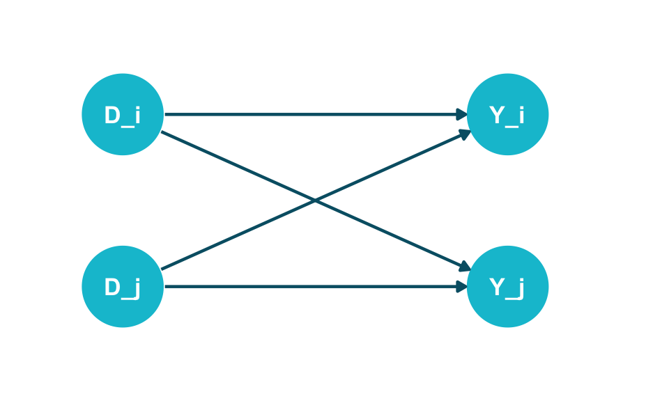
Two-sided market: treating buyer \(i\) affects seller \(j\)’s response, which affects buyer \(j\)’s outcome.

Concrete examples:

• Ride-share: surge pricing for treated riders displaces untreated riders’ wait times.
• Marketplace: new search ranking shifts shared supply between treated and untreated buyers.
• Social network: a feed change reaches untreated users via friend activity.

\(Y_i\) depends on \(D_j\) (\(j \neq i\)) — SUTVA fails.

User-level randomization estimates an effect diluted by spillover — toward zero in most marketplaces, away from zero in some. The next slide gives empirical evidence at Airbnb.

DAG slide. The graph has D_i and D_j (two units’ treatments) and Y_i and Y_j (two units’ outcomes), with cross-arrows D_i -> Y_j and D_j -> Y_i representing interference. In two-sided markets — Airbnb, DoorDash, Lyft — this is the rule, not the exception. The mechanism is supply-side: treated buyers and untreated buyers compete for the same supply (rides, listings, drivers), so giving treated buyers a better experience necessarily degrades the experience for untreated buyers. User-level random assignment underestimates the global treatment effect, sometimes by 30%+. The next slide quantifies this from the Airbnb meta-experiment.

Airbnb meta-experiment: cluster-randomization reduces SUTVA bias

Holtz et al. (2024) ran a meta-experiment at Airbnb: same intervention, randomized at two scales simultaneously.

• User-level randomization: each user independently treated or control.
• Cluster (market-level) randomization: entire geographic markets treated or control; spillovers contained within a market.

The empirical finding

The cluster-randomized estimate was ~32% larger than the user-level estimate.

Interpretation: user-level randomization underestimated the true global treatment effect by ~32% because untreated users absorbed some of the treatment’s positive externality.

The fix: when the unit of analysis is a marketplace, randomize at the marketplace level (geography, store, region) — not at the user level.

The empirical capstone of the SUTVA-violation arc. Holtz et al. 2024 is a Management Science paper that ran the same intervention at user-level and market-level simultaneously on Airbnb, then compared the estimated ATEs. The cluster-level estimate was 32% bigger — a huge SUTVA-bias-correction number. Practical takeaway: at any two-sided marketplace, if the intervention affects supply allocation, user-level randomization understates the global effect. Cluster-randomization (treat whole markets) is the standard fix. The next slide formalizes a related design — switchback — that handles spillover via time rather than geography.

Switchback designs: alternate global treatment across short time windows

When spillover is temporal (e.g., a dispatch algorithm changes the system-wide supply state for the next 30 minutes), splitting units doesn’t work — split time instead.

Switchback design (Bojinov, Simchi-Levi, and Zhao 2023): divide time into windows of length \(w\); in each window, set \(D = 1\) globally or \(D = 0\) globally; randomize the alternation.

Pros: handles cross-unit interference by treating the whole system; estimator is a simple windowed difference. Cons: temporal autocorrelation inflates the variance; carryover at window boundaries biases the estimate.

Switchback design definition. The picture is 24 colored tiles representing 30-minute windows alternating between D=1 and D=0 over a 12-hour period. The idea is to globally toggle the treatment on and off — every rider at time t gets the same policy — so within a window there is no interference and across windows the effect can be estimated as a windowed mean difference. The two costs are (1) windows are temporally autocorrelated, so the effective n is smaller than the number of windows, and (2) carryover at window boundaries (some riders span the boundary) biases the estimate slightly. The next slide gives DoorDash production numbers.

DoorDash uses 30-minute switchback windows for 30% faster iteration

DoorDash production deployment (Bojinov, Simchi-Levi, and Zhao 2023):

• Application: dispatch-algorithm A/B tests. Dispatch is a system-wide policy — assigning Dasher to order is interference-by-design.
• Window length: 30 minutes — long enough for the dispatch decision’s downstream effect to dissipate; short enough to log enough switches per day.
• Carryover correction: drop the first 5 minutes after each switch (the “warm-up” zone where the system is still equilibrating).

The throughput gain

Switchback designs let DoorDash run dispatch-algorithm experiments in 3–7 days versus the 2–3 weeks required by cluster (market-level) randomization — a 30% iteration-speed gain in their published 2023 case study.

Switchback has spread to Lyft (matching algorithms), Uber (surge pricing), and several food-delivery platforms. The reference design for any system-level policy test.

Production case study. DoorDash’s switchback deployment is the canonical industry case: 30-min windows on dispatch-algorithm tests, with 5-min carryover-correction drops. The 30% iteration-speed gain over cluster-randomization is the published Bojinov et al. number. Discuss in lecture: why didn’t they just cluster-randomize? Answer: cluster-randomization at city level means each city is one observation, so getting power on a small effect requires running for weeks. Switchback turns each 30-min window into a unit of analysis, which gives them thousands of observations per day. The trade-off is the carryover/autocorrelation cost — addressed in the next slide.

Carryover decay rates determine optimal window length

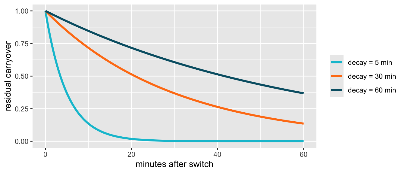
Hu and Wager (2022) show that the optimal switchback window length is a function of the carryover decay rate:

• If treatment effect decays in \(\sim 5\) minutes, 30-minute windows capture ~80% of “clean” variance.
• If decay is \(\sim 30\) minutes (slow carryover), 30-minute windows leave only ~50% clean; 2-hour windows are needed.
• If decay is \(> 1\) hour (very slow carryover), switchback becomes infeasible — fall back to cluster-randomization.

Diagnostic: estimate carryover from a pilot study (50 random switches, measure the first 30 minutes); choose window length so residual carryover at end-of-window is below 5%.

The technical pre-launch analysis required to choose a window length. Hu & Wager 2022 derive the optimal-window formula in closed form for a geometric-mixing model of carryover; the empirical implementation is to estimate the carryover half-life from a pilot study and then set window length to ~6 half-lives. The three-curve plot shows three regimes: fast decay (cyan) — switchback is great, slow decay (deep teal) — switchback fails, intermediate (orange) — works but with carryover-correction. Encourage students to run the pilot in their own data before committing to a switchback design.

Surrogate index: predict 63-day metric from 14-day proxies — Netflix

The long-horizon metric problem: business outcomes (retention, LTV, renewal) take months to observe; product decisions must happen in weeks.

Zhang et al. (2023) (Netflix): train a surrogate index \(\hat g(\mathbf{X}_{14d})\) to predict the 63-day metric from 14-day proxies; substitute \(\hat g\) for the true outcome at decision time.

The honest numbers

Reported Netflix results:

• 95% agreement between surrogate-based and 63-day-truth decision when both reject the null in the same direction.
• But only 65–79% recall of true launches — the surrogate misses 20–35% of real wins.
• And it occasionally falsely launches when the 14-day signal points in the wrong direction.

Use with caution. Surrogate methods are decision-time savers, not bias-free estimators. The right framing: surrogate trades 75% of decision quality for 5× decision speed.

Surrogate index is the most-asked-about A/B-testing topic of 2024-25 and the slide needs to land the honest caveat. The headline 95% agreement number is what Netflix advertises in the paper; the 65-79% recall number is the trade-off. Students will encounter surrogate methods at any tech company with long retention metrics, and they should leave knowing the methodology AND the honest cost. Frame it as “surrogate trades 75% of decision quality for 5× decision speed” — for some decisions that trade is worth it, for others it isn’t. The mathematics: surrogate-index estimation is fundamentally a prediction problem, not a causal-identification problem, so it’s only as good as the predictability of long-horizon from short-horizon outcomes.

When A/B breaks: a diagnostic flowchart

A one-page reference card for any experiment showing “interesting” effects:

Diagnostic question	Test	If failed → which slide / design?
1. Is the allocation as intended?	Chi-squared on counts vs. intended ratio.	Slide 37–38 (SRM): STOP and debug.
2. Could treated affect untreated?	DAG check: any \(D_i \to Y_j\) for \(i \neq j\)?	Slide 39–40: cluster-randomize or switchback.
3. Is interference temporal?	Pilot carryover study: 50 switches, 30-min decay.	Slide 41–43: switchback with tuned window.
4. Is the outcome too slow?	Decision-horizon \(\geq\) outcome-horizon?	Slide 44: surrogate index + caveat.

Discipline first. Estimation second. No SRM check → no estimator.

The Stack-4 takeaway flowchart. Every diagnostic question pairs with a test and a design fix. The questions are ordered by frequency in practice: SRM is the most common failure (1 in 10 to 1 in 16 experiments), interference is rare but huge when it bites (marketplaces, networks), temporal interference is rare but well-handled (switchback), and surrogate substitution is a niche fix. The closing tagline is the operational rule: no SRM check, no estimator. Tie this back to slide 36 (Twyman’s law) — diagnostic discipline first, statistical estimation second.

What’s Next

A/B testing is the easy case. Observational data is the rest of the course.

Final stack. Everything in S05 assumed randomization. When you cannot randomize — observational data, geo-experiments, long-horizon outcomes — the playbook changes radically. The forward-pointer slides preview five paths the course will take from here: HTE (S09), bandits (out of scope), geo-experiments (S11), Assignment II logistics, and a one-slide synthesis of S05’s main message. Keep this stack tight — five slides, ~5 minutes — to leave time for student questions at the end of the lecture.

Treatment effects vary — and tech firms exploit it: HTE in production

The ATE is a single number. The real treatment effect is a function \(\tau(x)\) of pre-treatment features. Tech firms increasingly exploit this:

• Netflix HTE blog series (2024): firmware-dependent updates show different effects on smart-TV firmware versions; the firm rolls out the update only on firmwares where the effect is positive.
• Country-level homepage variants: same A/B test, different ATE in 50+ countries → ship per-country.
• Push-vs-email contact strategy: HTE on user-tenure variables → personalized contact policy.

Session 9 turns HTE into a formal estimator

In Session 9: Treatment Effect Heterogeneity, we cover causal forests, meta-learners, and the R-learner — the formal machinery that estimates \(\tau(x)\) from experimental data and supports per-segment ship decisions.

HTE teaser. Most A/B tests stop at the ATE — a single average number across all users. But the real per-user effect varies with covariates, and tech firms increasingly exploit this by rolling out only to user segments where the effect is positive. Netflix’s HTE blog series is the cleanest published case. Session 9 introduces the formal estimators (causal forests, meta-learners, R-learner). Keep this slide short: the message is “ATE is only the start; per-segment ship decisions are the future.”

Bandits vs. A/B: when exploration trumps significance

Multi-armed bandits trade off exploration (try every arm to learn) against exploitation (route traffic to the best arm so far).

Bandit case studies (out of course scope)

• Spotify 2025: contextual-bandit personalization for playlist recommendations.
• Stitch Fix: bandits for inventory-recommendation strategy.
• News publishers: Thompson Sampling for headline selection (3–10× faster than A/B at the same regret budget).

When A/B vs. when bandit:

• A/B: one-shot launch decisions; need to interpret the effect.
• Bandit: continuous-decision settings where you want to act on the effect, not interpret it.

Bandits are out of scope for this course — the formal theory needs a reinforcement-learning toolkit. But every year students ask, “Why not bandits for everything?” The answer: A/B testing remains the right tool when the value of understanding the effect exceeds the cost of not exploiting it during the experiment.

The annual “why not bandits” question, pre-empted. Bandits trade interpretability for exploitation: they route more traffic to the best arm as soon as evidence accumulates, which is great for ad-serving or recommendation but bad for “what is the actual effect of this feature on engagement.” For one-shot launch decisions (most product A/B tests), interpretability matters and you should pay the cost of equal allocation. For continuous-decision settings (which ad creative to show), you should bandit. Flag this slide as out-of-course-scope — full bandit treatment requires reinforcement-learning machinery beyond what we cover.

Geo-experiments: when individual randomization is impossible → S11

Some interventions cannot be randomized at user level:

• Television and OOH advertising: ads are visible to everyone in a market; assignment is geographic by construction.
• Marketing mix tests: spend changes across countries or DMAs, not individual users.
• Regulatory or pricing rollouts: same price for everyone in a city.

Geo-experiment: randomize markets (DMAs, cities, countries) to treatment vs. control; estimate the effect as the difference in market-level outcomes, adjusting for market-level pre-treatment trends.

Session 11 covers the analysis method

When you have very few markets (5 treated vs. 5 control), naive difference-in-means is underpowered. Synthetic controls (Abadie et al.) construct a weighted control from the donor pool. That is Session 11.

Geo-experiment teaser. The motivating problem: some interventions are infeasible to randomize at the individual level — TV ads, citywide pricing, regulatory rollouts. The design fix is to randomize at the market level (geographies, DMAs, countries). But because markets are correlated and few in number, naive market-level mean differences have low power. The solution is the synthetic control method — Session 11’s main topic — which constructs a counterfactual control from a weighted combination of donor markets. Tease the connection; don’t deliver the method.

Assignment II covers S04 + S05 (due 2026-05-31)

Assignment II is the second of five graded assignments (20% of final grade). Released after today’s lecture; due Sunday 31 May 2026, 23:59.

Assignment II — Online A/B-Test Reanalysis

You will be given a real or realistically simulated A/B-test dataset (~50,000 users, 2 arms, 14 days). Your task:

1. SRM diagnostic — chi-squared check on assignment counts.
2. OEC + guardrails — define and report.
3. CUPED estimator — implement; report variance reduction vs. naive.
4. One inference mode — fixed-horizon, sequential, or Bayesian. Justify the choice.
5. Brief HTE exploration — segment by 1 covariate; report whether segment-level effects diverge.

Submission: rendered Quarto report (R or Python), code embedded.

The 15-minute paper quiz at the lecture session on Monday 2026-06-01 gates the grade — you must score ≥ 50% on the quiz or your report grade is capped at 60%. Quiz draws directly from today’s diagnostic and inference content (SRM, CUPED, peeking).

The assignment hook. The five-part structure mirrors the five stacks of today’s lecture: motivation (OEC), variance reduction (CUPED), inference mode choice, what-breaks (SRM), and a preview of HTE. Encourage students to start with the SRM check — if the assignment dataset has SRM, the rest of the analysis is uninterpretable. The quiz gate is the assessment-design contract from earlier in the semester: paper quiz on the Tuesday after submission, 50% threshold, otherwise grade capped at 60%. Quiz content is restricted to operational diagnostics (SRM, CUPED, peeking) — material students can revise from this slide deck alone.

Five tools, one decision: trust the OEC, trust the diagnostics, trust the math

The session in three lines:

• Variance reduction → more experiments per quarter. (CUPED, CUPAC, MLRATE.)

• The right inference mode → defensible decisions under peeking. (Sequential, Bayesian, alpha-spending.)

• SUTVA discipline → unbiased estimates at scale. (SRM check, cluster randomization, switchback, surrogate.)

Three families of tools, one operational discipline: define the OEC, run the diagnostics, choose the inference mode — in that order.

Next session: observed confounding — when you cannot randomize, what do you do instead?

Final synthesis slide. Three families of tools — variance reduction, inference modes, SUTVA discipline — each tied to a single decision pillar. The operational order matters: OEC first (you can’t measure what you didn’t define), diagnostics second (no SRM, no estimator), inference mode third (peeking-safe inference on a clean experiment). End with the explicit transition to Session 6: everything in S05 assumed randomization; when you cannot randomize (observational data), the entire playbook changes. That is Session 6’s territory.

References

Berman, Ron, and Christophe Van den Bulte. 2022. “False Discovery in A/B Testing.” Management Science 68 (9): 6762–82. https://doi.org/10.1287/mnsc.2021.4207.

Biswas, Dipayan, Annika Abell, and Roger Chacko. 2024. “Curvy Digital Marketing Designs: Virtual Elements with Rounded Shapes Enhance Online Click-Through Rates.” Journal of Consumer Research 51 (3): 552–75. https://doi.org/10.1093/jcr/ucad078.

Bojinov, Iavor, David Simchi-Levi, and Jinglong Zhao. 2023. “Design and Analysis of Switchback Experiments.” Management Science 69 (7): 3759–77. https://doi.org/10.1287/mnsc.2022.4583.

Deng, Alex, Ya Xu, Ron Kohavi, and Toby Walker. 2013. “Improving the Sensitivity of Online Controlled Experiments by Utilizing Pre-Experiment Data.” In Proceedings of the Sixth ACM International Conference on Web Search and Data Mining (WSDM), 123–32. https://doi.org/10.1145/2433396.2433413.

Fabijan, Aleksander, Jayant Gupchup, Somit Gupta, Jeff Omhover, Wen Qin, Lukas Vermeer, and Pavel Dmitriev. 2019. “Diagnosing Sample Ratio Mismatch in Online Controlled Experiments: A Taxonomy and Rules of Thumb for Practitioners.” In Proceedings of the 25th ACM SIGKDD International Conference on Knowledge Discovery and Data Mining (KDD), 2156–64. https://doi.org/10.1145/3292500.3330722.

Guo, Yongyi, Dominic Coey, Mikael Konutgan, Wenting Li, Chris Schoener, and Matt Goldman. 2021. “Machine Learning for Variance Reduction in Online Experiments.” In Advances in Neural Information Processing Systems 34 (NeurIPS). https://proceedings.neurips.cc/paper/2021/hash/488b084119a1c7a4950f00706ec7ea16-Abstract.html.

Holtz, David, Felipe Lobel, Ruben Lobel, Inessa Liskovich, and Sinan Aral. 2024. “Reducing Interference Bias in Online Marketplace Experiments Using Cluster Randomization: Evidence from a Pricing Meta-Experiment on Airbnb.” Management Science 71 (1). https://doi.org/10.1287/mnsc.2020.01157.

Howard, Steven R., Aaditya Ramdas, Jon McAuliffe, and Jasjeet Sekhon. 2021. “Time-Uniform, Nonparametric, Nonasymptotic Confidence Sequences.” The Annals of Statistics 49 (2): 1055–80. https://doi.org/10.1214/20-AOS1991.

Hu, Yuchen, and Stefan Wager. 2022. “Switchback Experiments Under Geometric Mixing.” https://arxiv.org/abs/2209.00197.

Kohavi, Ron, Alex Deng, Brian Frasca, Roger Longbotham, Toby Walker, and Ya Xu. 2012. “Trustworthy Online Controlled Experiments: Five Puzzling Outcomes Explained.” In Proceedings of the 18th ACM SIGKDD International Conference on Knowledge Discovery and Data Mining (KDD), 786–94. https://doi.org/10.1145/2339530.2339653.

Kohavi, Ron, Jakub Linowski, Lukas Vermeer, Fabrice Boisseranc, Joachim Furuseth, Andrew Gelman, Guido Imbens, and Ravikiran Rajagopal. 2026. “Power Analysis Is Essential: High-Powered Tests Suggest Minimal to No Effect of Rounded Shapes on Click-Through Rates.” Econ Journal Watch 23 (1): 138–60.

Kohavi, Ron, Diane Tang, and Ya Xu. 2020. Trustworthy Online Controlled Experiments: A Practical Guide to a/b Testing. Cambridge University Press. https://doi.org/10.1017/9781108653985.

Larsen, Nicholas, Jonathan Stallrich, Srijan Sengupta, Alex Deng, Ron Kohavi, and Nathaniel T. Stevens. 2024. “Statistical Challenges in Online Controlled Experiments: A Review of A/B Testing Methodology.” The American Statistician 78 (2): 135–49. https://doi.org/10.1080/00031305.2023.2257237.

Lin, Winston. 2013. “Agnostic Notes on Regression Adjustments to Experimental Data: Reexamining Freedman’s Critique.” Annals of Applied Statistics 7 (1): 295–318.

Lindon, Michael, Dae Woong Ham, Martin Tingley, and Iavor Bojinov. 2024. “Anytime-Valid Linear Models and Regression-Adjusted Causal Inference in Randomized Experiments.” https://arxiv.org/abs/2210.08589.

Waudby-Smith, Ian, and Aaditya Ramdas. 2024. “Estimating Means of Bounded Random Variables by Betting.” Journal of the Royal Statistical Society: Series B 86 (1): 1–27. https://doi.org/10.1093/jrsssb/qkad009.

Zhang, Vickie, Michael Zhao, Maria Dimakopoulou, Anh Le, and Nathan Kallus. 2023. “Evaluating the Surrogate Index as a Decision-Making Tool Using 200 A/B Tests at Netflix.” https://arxiv.org/abs/2311.11922.

Thank you for your attention!
	www.startupengineer.io/team/ihl/ christoph-ihl christophihl