3. Causal Graphs and Discovery

Causal Data Science for Business Analytics

Christoph Ihl

Hamburg University of Technology

Tuesday, 28. April 2026

The Backdoor Criterion

The backdoor criterion translates d-separation into an actionable adjustment strategy

Transition to the backdoor criterion. So far we can check whether two variables are d-separated given a conditioning set. But the practical question is the reverse: given a treatment D and outcome Y, which variables should we condition on to identify the causal effect? The backdoor criterion provides a sufficient graphical condition that answers this question. It is the most commonly used identification strategy in applied causal inference.

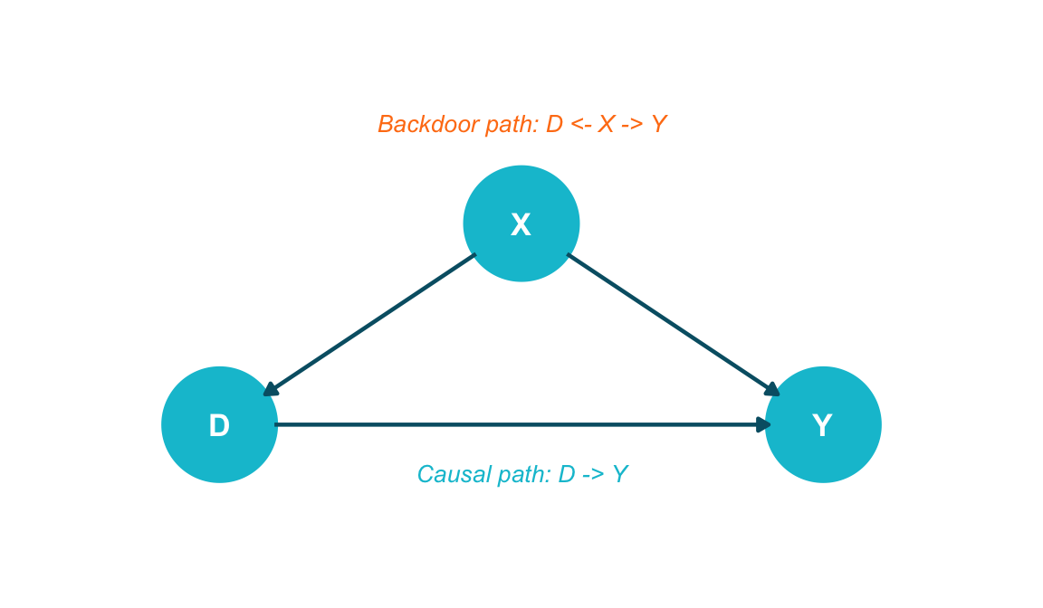
Backdoor paths are the source of confounding bias

A backdoor path from \(D\) to \(Y\) is any path that starts with an arrow into \(D\) (i.e., \(D \leftarrow \ldots\)).

These paths are non-causal — they transmit spurious association due to confounding, not genuine causal effects.

A causal (directed) path from \(D\) to \(Y\) follows arrows forward: \(D \rightarrow \ldots \rightarrow Y\).

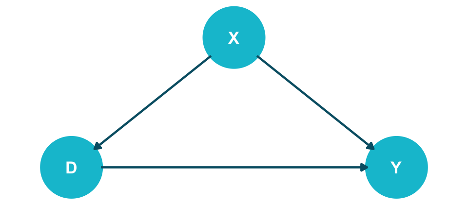
Business example: Marketing spend (\(D\)) \(\rightarrow\) Revenue (\(Y\)), with company size (\(X\)) as confounder: \(D \leftarrow X \rightarrow Y\). Larger firms spend more on marketing AND earn more revenue.

library(ggdag)
library(ggplot2)

coord_dag <- list(
  x = c(D = 0, X = 0.5, Y = 1),
  y = c(D = 0, X = 0.5, Y = 0)
)

dag <- dagify(D ~ X,
              Y ~ D,
              Y ~ X,
              coords = coord_dag)

dag_data <- dag |> tidy_dagitty()

dag_data |>
  ggplot(aes(x = x, y = y, xend = xend, yend = yend)) +
  geom_dag_point(colour = "#00C1D4", size = 22) +
  geom_dag_edges(edge_colour = "#005e73", edge_width = 0.8) +
  geom_dag_text(colour = "white", size = 4.5, fontface = "bold") +
  annotate("text", x = 0.5, y = -0.12, label = "Causal path: D -> Y",
           colour = "#00C1D4", size = 3.5, fontface = "italic") +
  annotate("text", x = 0.5, y = 0.75, label = "Backdoor path: D <- X -> Y",
           colour = "#FF7E15", size = 3.5, fontface = "italic") +
  expand_limits(x = c(-0.2, 1.2), y = c(-0.3, 0.9)) +
  coord_cartesian(clip = "off") +
  theme_dag(legend.position = "none")

Define the two types of paths that connect treatment and outcome. Causal paths follow arrows from D toward Y — these represent the genuine causal effect we want to measure. Backdoor paths start with an arrow into D, flowing through common causes. These are the confounding paths. The goal of causal identification is to block all backdoor paths while leaving the causal paths intact. In the marketing example, budget allocation determines both how much is spent on marketing and revenue through other channels. The observed correlation between marketing spend and revenue conflates the causal effect with the confounding through budget allocation.

The backdoor criterion tells you exactly what to condition on

Backdoor Criterion (Pearl, 1993)

A set of variables \(X\) satisfies the backdoor criterion relative to \((D, Y)\) if:

1. \(X\) blocks all backdoor paths from \(D\) to \(Y\)
2. \(X\) contains no descendant of \(D\)

If \(X\) satisfies the backdoor criterion, then the causal effect is identified by the adjustment formula from Session 01 — now with a graphical justification for choosing \(X\) (Pearl 2009):

\[\tau = \sum_x \Big(\mathbb{E}[Y \mid D = 1, X = x] - \mathbb{E}[Y \mid D = 0, X = x]\Big)\,\textcolor{#FF7E15}{P(X = x)}\]

The backdoor criterion guarantees that this observational formula identifies a causal effect — averaging the conditional contrasts with the natural weight \(\textcolor{#FF7E15}{P(X)}\), the orange weight from the previous derivation. Two frameworks formalize what that causal quantity is — derivation on the next slide.

The backdoor criterion is Pearl’s graphical condition for identifying causal effects via covariate adjustment. Condition 1 says we must block all non-causal paths between D and Y. Condition 2 says we must not condition on descendants of D, which could block part of the causal effect or open collider paths. If both conditions are met, the do-calculus tells us that the interventional distribution equals the adjustment formula. The key insight: this is exactly the same formula we derived from potential outcomes in Session 01 under conditional exchangeability. The backdoor criterion provides the graphical condition under which conditional exchangeability holds. The formula looks the same, but now we have a systematic way to choose X rather than relying on intuition.

Backdoor adjustment connects DAGs to potential outcomes

do-notation (Pearl):

Step 1 — backdoor criterion ⇒ truncated factorization at \(D = d\): \[P(X, Y \mid do(D = d)) = P(Y \mid D = d, X)\,\textcolor{#FF7E15}{P(X)}\]

Step 2 — sum over \(x\) (graph surgery preserves the kernel): \[E[Y \mid do(D = d)] = \sum_x E[Y \mid D = d, X = x]\,\textcolor{#FF7E15}{P(X = x)}\]

Natural weight \(\textcolor{#FF7E15}{P(X)}\) — the single-confounder argument generalized to a sufficient set \(X\).

Potential outcomes (Rubin):

Step 1 — conditional exchangeability \(Y(d) \perp\!\!\!\perp D \mid X\): \[E[Y(d) \mid X = x] = E[Y \mid D = d, X = x]\]

Step 2 — law of total expectation over \(\textcolor{#FF7E15}{P(X)}\): \[E[Y(d)] = \sum_x E[Y \mid D = d, X = x]\,\textcolor{#FF7E15}{P(X = x)}\]

Natural weight \(\textcolor{#FF7E15}{P(X)}\) — emerges from marginalizing the population.

Bridge: \(X\) satisfies the backdoor criterion in the DAG \(\iff\) \((Y(1), Y(0)) \perp\!\!\!\perp D \mid X\) (conditional exchangeability) (Hünermund and Bareinboim 2023). Two routes, same kernel \(E[Y \mid D = d, X]\), same orange weight \(\textcolor{#FF7E15}{P(X)}\). DAGs help find \(X\); potential outcomes define the estimand.

With the do-operator derivation now in hand, both routes can be made explicit. do-side: the backdoor criterion guarantees that, in the mutilated graph \(G_{\overline{D}}\), the truncated factorization preserves the kernel \(P(Y \mid D = d, X)\) from the observational graph. Marginalizing \(X\) with the natural weight \(P(X)\) yields the adjustment formula — exactly the same move as in the single-confounder slide, now for a sufficient set \(X\). PO-side: conditional exchangeability \(Y(d) \perp\!\!\!\perp D \mid X\) lets us replace the unobservable counterfactual \(E[Y(d) \mid X]\) with the observable \(E[Y \mid D = d, X]\). Then law of total expectation marginalizes \(X\) with \(P(X)\). Both routes arrive at the same kernel multiplied by the same natural weight — the orange weight from the previous derivation — and the equivalence between them is the bridge: the backdoor criterion is a graphical sufficient condition for conditional exchangeability. The frameworks are complementary, not competing: DAGs give a systematic way to determine which \(X\) to condition on; potential outcomes give a precise definition of the causal estimand and the assumptions under which it is identified. Hünermund and Bareinboim (2023) provide a thorough treatment of this connection in the econometrics context.

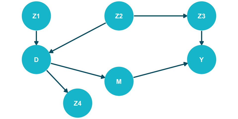
Worked example: finding adjustment sets in a complex DAG

library(ggdag)
library(ggplot2)

coord_dag <- list(
  x = c(Z1 = 0, Z2 = 0.5, D = 0, M = 0.5, Y = 1, Z3 = 1, Z4 = 0.25),
  y = c(Z1 = 1, Z2 = 1, D = 0.5, M = 0.25, Y = 0.5, Z3 = 1, Z4 = 0)
)

dag <- dagify(
  D ~ Z1,
  D ~ Z2,
  Z3 ~ Z2,
  M ~ D,
  Y ~ M,
  Y ~ Z3,
  Z4 ~ D,
  coords = coord_dag
)

dag |>
  ggplot(aes(x = x, y = y, xend = xend, yend = yend)) +
  geom_dag_point(colour = "#00C1D4", size = 20) +
  geom_dag_edges(edge_colour = "#005e73", edge_width = 0.8) +
  geom_dag_text(colour = "white", size = 3.5, fontface = "bold") +
  expand_limits(x = c(-0.1, 1.1), y = c(-0.1, 1.1)) +
  coord_cartesian(clip = "off") +
  theme_dag(legend.position = "none") +
  theme(plot.margin = margin(-5, 0, -5, 0))

• R
• Python

library(dagitty)
dag <- dagitty("dag{
  Z1 -> D; Z2 -> D; Z2 -> Z3;
  D -> M -> Y; Z3 -> Y; D -> Z4
}")
print(adjustmentSets(dag, exposure = "D", outcome = "Y"))

{ Z3 }
{ Z2 }

from pgmpy.base import DAG
from pgmpy.inference import CausalInference

dag = DAG([
    ("Z1", "D"), ("Z2", "D"), ("Z2", "Z3"),
    ("D", "M"), ("M", "Y"), ("Z3", "Y"), ("D", "Z4")
])
ci = CausalInference(dag)
print(ci.get_all_backdoor_adjustment_sets("D", "Y"))

frozenset({frozenset({'Z3'}), frozenset({'Z2'})})

Backdoor paths from \(D\) to \(Y\):

1. \(D \leftarrow Z2 \rightarrow Z3 \rightarrow Y\) (open fork at Z2)
2. \(D \leftarrow Z1 \; \ldots\) (Z1 has no path to Y — dead end)

Only path 1 needs blocking. Exclude \(M\) (mediator — conditioning blocks the causal path) and \(Z4\) (descendant of \(D\) — may open collider paths).

Multiple valid sets exist: \(\{Z2\}\), \(\{Z3\}\), \(\{Z2, Z3\}\), \(\{Z1, Z2\}\), etc. The minimal sufficient set is often preferred (fewer variables \(=\) less variance).

Walk through the adjustment set analysis. The DAG has one genuine backdoor path: D gets Z2’s influence, and Z2 also influences Y through Z3. Z1 has an arrow into D but no path to Y, so it does not create a backdoor path. To satisfy the backdoor criterion, we need to block the Z2-Z3 path. We can do this by conditioning on Z2 (the fork) or on Z3 (the chain). Both are valid. We cannot include M (mediator, descendant of D) or Z4 (another descendant of D). The adjustmentSets function computes all valid minimal sets. In practice, the choice among valid sets depends on measurement quality and sample size considerations. The point is that the DAG gives you all valid options.

Common mistakes: four DAG patterns that trap analysts

1. Adjusting for a mediator

\(D \rightarrow M \rightarrow Y\)

Conditioning on \(M\) blocks the causal pathway, underestimating the total effect.

2. Adjusting for a collider

\(D \rightarrow Z \leftarrow Y\)   (conditioning on \(Z\))

Opens a spurious path, creating bias where none existed.

3. Adjusting for a descendant of treatment

\(D \rightarrow Z \rightarrow \ldots\)

Partially blocks the causal pathway and may open collider paths.

4. Failing to adjust for a confounder

\(D \leftarrow W \rightarrow Y\)   (not conditioning on \(W\))

Leaves the backdoor path open — the classic omitted variable bias.

All four mistakes are prevented by drawing a DAG and applying the backdoor criterion before running any regression.

This slide catalogs the four most common adjustment errors in applied work. Mistake 1 is the overcontrol trap: if you adjust for a mediator, you block part of the very effect you are trying to measure. Mistake 2 is the collider trap we saw earlier. Mistake 3 is a subtler version: descendants of D may be mediators or may open collider paths. Mistake 4 is the classic omitted variable problem. The unifying message: every one of these mistakes can be diagnosed and prevented by a DAG. Draw the graph first, apply the backdoor criterion, and only then decide which variables to include in your model. This is why graphical causal models are not just theoretical elegance but practical necessity.

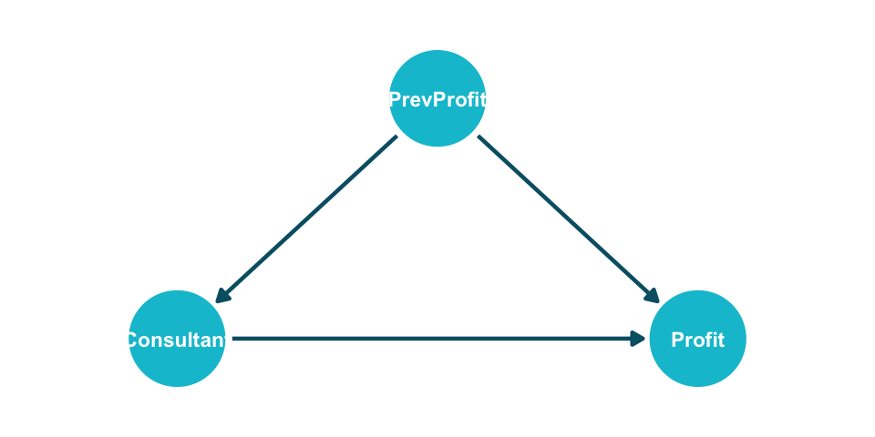
Applied example: estimating the effect of consulting on profits

• R
• Python

library(ggdag); library(dagitty)

dag <- dagify(Consultant ~ PrevProfit,
              Profit ~ Consultant + PrevProfit,
              exposure = "Consultant",
              outcome = "Profit")

ggdag(dag) # plot DAG
adjustmentSets(dag) # find valid sets

from pgmpy.base import DAG
from pgmpy.inference import CausalInference

dag = DAG([("PrevProfit", "Consultant"),
           ("Consultant", "Profit"),
           ("PrevProfit", "Profit")])

ci = CausalInference(dag)
ci.get_all_backdoor_adjustment_sets(
    "Consultant", "Profit")

{ PrevProfit }

• R
• Python

library(dplyr)

# Simulate data
set.seed(42); n <- 1000
previous_profit <- rnorm(n, 5, 2) + 2 * rbinom(n, 1, 0.3)
consultant <- rbinom(n, 1, ifelse(previous_profit >
                     median(previous_profit), 0.75, 0.25))
profit <- 0.85 * previous_profit + 1 * consultant +
          rnorm(n, 0, 0.1)

# Naive vs. adjusted ATE
naive <- mean(profit[consultant == 1]) -
         mean(profit[consultant == 0])
stratum <- ntile(previous_profit, 4)
adjusted <- mean(tapply(seq_len(n), stratum, \(i)
  mean(profit[i][consultant[i] == 1]) -
  mean(profit[i][consultant[i] == 0])))

import numpy as np
import pandas as pd

np.random.seed(42); n = 1000
prev = np.random.normal(5, 2, n) + 2 * np.random.binomial(1, 0.3, n)
prob = np.where(prev > np.median(prev), 0.75, 0.25)
cons = np.random.binomial(1, prob)
profit = 0.85 * prev + 1 * cons + np.random.normal(0, 0.1, n)

# Naive vs. adjusted ATE
naive = profit[cons == 1].mean() - profit[cons == 0].mean()
df = pd.DataFrame({"prev": prev, "cons": cons, "profit": profit})
df["q"] = pd.qcut(df["prev"], 4, labels=False)
adj = df.groupby("q").apply(
    lambda g: g.loc[g.cons == 1, "profit"].mean() -
              g.loc[g.cons == 0, "profit"].mean()).mean()

Naive ATE (no adjustment):       2.32 

Adjusted ATE (stratified):        0.99 

True causal effect:               1.00

Previous profit confounds the comparison: profitable firms hire more consultants AND earn more. The naive estimate is biased upward; adjusting recovers the true effect.

This applied example ties everything together. The DAG encodes a simple business story: companies with higher previous profits are more likely to hire consultants (selection effect), and previous profits also predict current profits (persistence). The naive comparison of means between consultant and non-consultant companies overestimates the effect because it conflates the consulting effect with the confounding by previous profit. The stratified estimate, which adjusts for previous profit using quartile bins, recovers the true causal effect of approximately 1.0. The data-generating process has a true effect of exactly 1.0, so students can verify that the adjustment works. This is a miniature version of what researchers do with real observational data, and the backdoor criterion told us exactly which variable to adjust for.

The Frontdoor Criterion

The backdoor criterion is powerful — but not complete. When confounders are unobserved, no ML algorithm will ever solve this problem.

Transition into the frontdoor criterion. The backdoor criterion handles the most common identification scenario: all confounders are observed. But what if the confounder is unobserved? Then no amount of data and no ML algorithm can recover the causal effect by stratification — the variable you would need to condition on simply isn’t in your dataset. The frontdoor criterion is the answer to this exact problem: when a mediator captures the entire causal pathway from treatment to outcome, the effect is still identified, even though the confounder remains hidden. It is the second major identification strategy in graphical causal models, on equal footing with the backdoor.

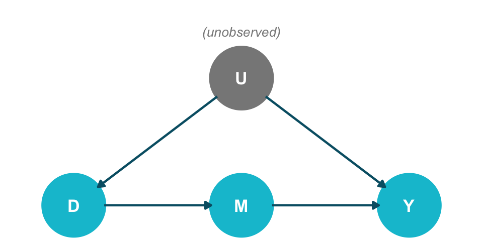
Frontdoor adjustment: identifying effects through a mediator

Example: Social media (\(D\)) \(\rightarrow\) word-of-mouth (\(M\)) \(\rightarrow\) sales (\(Y\)), brand awareness (\(U\)) unobserved.

library(ggdag)
library(ggplot2)

coord_dag <- list(
  x = c(D = 0, M = 0.5, Y = 1, U = 0.5),
  y = c(D = 0, M = 0, Y = 0, U = 0.6)
)

dag <- dagify(M ~ D,
              Y ~ M,
              D ~ U,
              Y ~ U,
              coords = coord_dag)

dag_data <- dag |> tidy_dagitty()
dag_data$data$colour <- ifelse(dag_data$data$name == "U", "#888888", "#00C1D4")

dag_data |>
  ggplot(aes(x = x, y = y, xend = xend, yend = yend)) +
  geom_dag_point(aes(colour = colour), size = 22) +
  scale_colour_identity() +
  geom_dag_edges(edge_colour = "#005e73", edge_width = 0.8) +
  geom_dag_text(colour = "white", size = 4.5, fontface = "bold") +
  annotate("text", x = 0.5, y = 0.82, label = "(unobserved)",
           colour = "#888888", size = 3.5, fontface = "italic") +
  expand_limits(x = c(-0.1, 1.1), y = c(-0.1, 0.9)) +
  coord_cartesian(clip = "off") +
  theme_dag(legend.position = "none") +
  theme(plot.margin = margin(-5, 0, -5, 0))

• \(U\) is unobserved — backdoor adjustment is impossible.
• But \(M\) fully mediates the effect of \(D\) on \(Y\): every causal path from \(D\) to \(Y\) runs through \(M\).
• Idea: isolate the causal flow that travels along the directed paths \(D \rightarrow M \rightarrow Y\), splitting an un-identifiable problem into two identifiable pieces.
• \(M\) satisfies the frontdoor criterion — the second major identification strategy.

This slide answers when the frontdoor criterion applies. The DAG is the canonical frontdoor structure: a treatment D, a mediator M, an outcome Y, and an unobserved common cause U of D and Y. The backdoor path D ← U → Y is open because we cannot condition on U. Backdoor adjustment is therefore impossible. But the directed causal path from D to Y goes entirely through M. The key insight is that the causal effect of D on Y is just whatever signal travels through the mediator — if we can separately identify D → M and M → Y, we can compose them. The business example: we cannot observe brand awareness, but if we can measure word-of-mouth reach as a mediator, we can still identify the causal effect of social media spending on sales. Next slide: the three-step procedure that does the composition.

Frontdoor in three steps

Step 1: Identify \(D \rightarrow M\).

The only backdoor path \(D \leftarrow U \rightarrow Y \leftarrow M\) contains a collider at \(Y\). Blocked. So \[P(M \mid do(D = d)) = P(M \mid D = d).\]

Step 2: Identify \(M \rightarrow Y\).

Backdoor path: \(M \leftarrow D \leftarrow U \rightarrow Y\). Condition on \(D\) to block it. So \[P(Y \mid do(M = m)) = \sum_{d} P(Y \mid M = m, D = d)\,P(D = d).\]

Step 3: Combine the two do-free quantities.

Sum over all realizations \(m\) of \(P(M \mid do(D = d))\): \[P(Y \mid do(D = d)) = \sum_{m} P(M = m \mid D = d) \sum_{d'} P(Y \mid M = m, D = d')\,P(D = d').\]

Walk through the three steps carefully. Step 1: the effect of D on M is identified because the only backdoor path D ← U → Y ← M contains a collider at Y, which is naturally blocked when we don’t condition on Y. So P(M|do(D)) equals the observational P(M|D) — no adjustment needed. Step 2: the effect of M on Y is identified by adjusting for D, which blocks the backdoor path M ← D ← U → Y, and weighting by the natural marginal P(D = d). Step 3: combine the two by the chain rule, summing over all realizations of the mediator. The frontdoor criterion is less commonly applicable than the backdoor — it requires a complete mediator, which is a strong structural assumption — but when it holds, it lets you identify causal effects despite unobserved confounding. The full algebraic proof, with each d-separation justification, is in the lecture notes.

Frontdoor criterion: theorem and definition

Combining the do-free quantities yields a closed-form expression in only observed variables:

Theorem: Frontdoor Adjustment

If \((D, M, Y)\) satisfies the frontdoor criterion and positivity, then \[P(Y \mid do(D = d)) = \sum_{m} P(M = m \mid D = d) \sum_{d'} P(Y \mid M = m, D = d')\,P(D = d').\]

Definition: Frontdoor Criterion

A variable \(M\) satisfies the frontdoor criterion relative to \((D, Y)\) if:

1. \(M\) completely mediates the effect of \(D\) on \(Y\) — every directed path from \(D\) to \(Y\) passes through \(M\).
2. There is no unblocked backdoor path from \(D\) to \(M\).
3. All backdoor paths from \(M\) to \(Y\) are blocked by \(D\).

The theorem packages the three-step procedure into one formula in only observed variables — D, M, Y — even though U remains hidden. The outer sum reweights conditional outcomes by the natural marginal P(D = d’). The definition makes precise the structural assumptions: the mediator must capture the entire causal mechanism (no direct D → Y arrow that bypasses M), there must be no unblocked backdoor into the mediator, and conditioning on D must block any backdoor from the mediator to the outcome. All three conditions are visible in the canonical DAG. The full step-by-step proof, with each d-separation justification, is in the lecture notes.

do-Calculus and the Causal Hierarchy

Three rules systematically remove do-operators from any causal expression

Transition to the three rules. The goal of do-calculus is mechanical: given a causal query like P(Y|do(D)), apply rules that convert do-expressions into purely observational expressions. Each rule handles a different situation — irrelevant observations, exchanging interventions for observations, and dropping irrelevant interventions. If the rules succeed in removing all do-operators, the effect is identified. The key tool is graph surgery: modifying the DAG by deleting specific arrows, then checking d-separation in the modified graph.

Two surgeries for the rules: \(G_{\overline{X}}\) and \(G_{\underline{X}}\)

Observational graph \(G\):

When we simply observe \(D\), all arrows remain. \(D\) is determined by its causes (including confounders).

Mutilated graph \(G_{\overline{D}}\):

When we intervene on \(D\) (set \(D = d\)), we delete all arrows into \(D\). The intervention replaces whatever normally determines \(D\).

The do-operator is concrete: \(P(Y \mid do(D = d))\) is simply \(P(Y \mid D = d)\) in the mutilated graph \(G_{\overline{D}}\). Graph surgery severs the confounding, making \(D\) independent of \(X\). This is exactly what an RCT does in practice.

Two surgeries, two notations: \(G_{\overline{X}}\) deletes arrows into \(X\) (used for Rules 1 & 3); \(G_{\underline{X}}\) deletes arrows out of \(X\) (used in Rule 2 to test whether observation can replace intervention).

Graph surgery is the graphical counterpart of an intervention. In the observational graph, D is caused by X (the confounder), so observing D tells us something about X, which biases our estimate of D’s effect on Y. When we intervene on D, we set it to a specific value regardless of X. Graphically, this means deleting all arrows into D. In the mutilated graph, D has no parents, so it is independent of X. The do-operator simply computes regular conditional probabilities in this modified graph. The key insight: an RCT does exactly this. Randomization breaks the link between the treatment and its natural causes. The mutilated graph makes this idea precise. The fragment introduces both notations students will need: the over-bar deletes incoming arrows (intervention), the under-bar deletes outgoing arrows (used in Rule 2 to check whether intervention can be exchanged for observation).

Rule 1: Irrelevant observations can be dropped

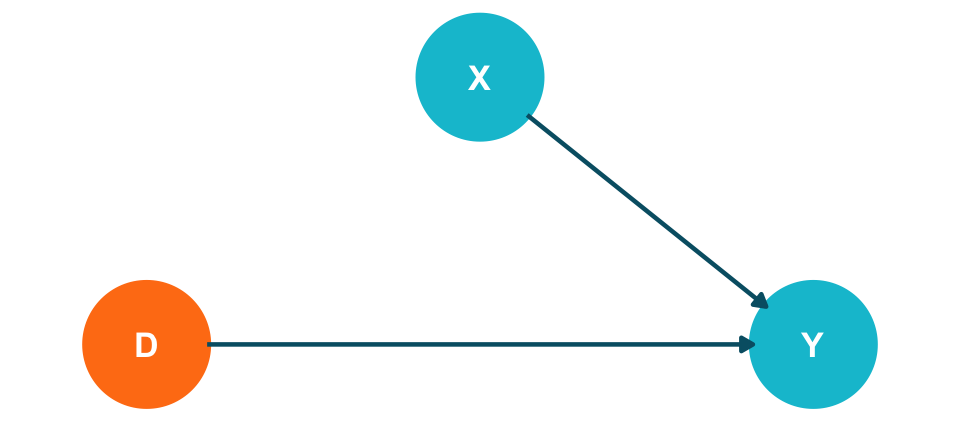
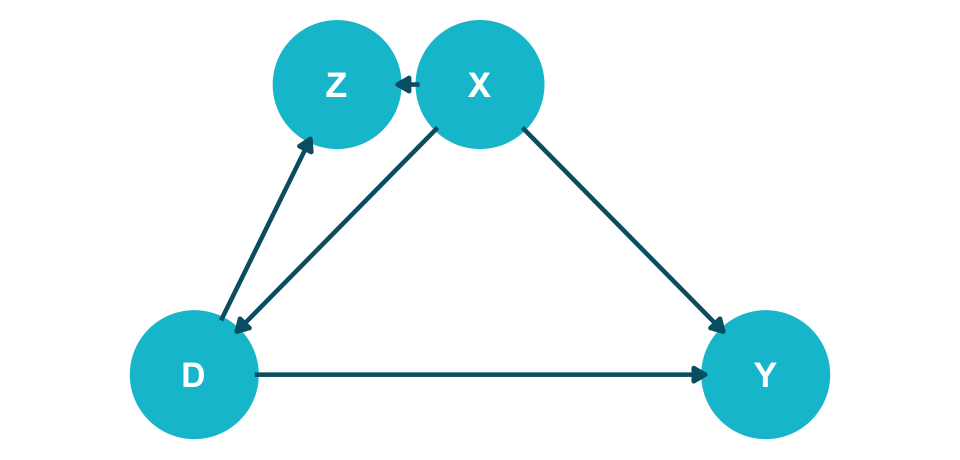
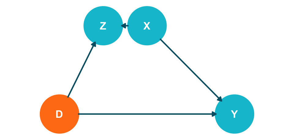
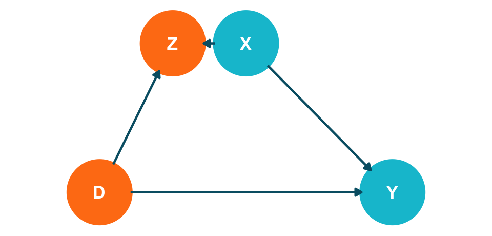
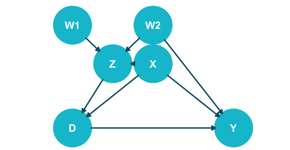
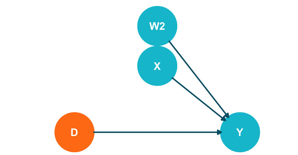
Rule: If \(Y \perp\!\!\!\perp_{G_{\overline{D}}} Z \mid D, X\), then \(P(Y \mid do(D), Z, X) = P(Y \mid do(D), X)\)

Check in \(G_{\overline{D}}\) (delete arrows into \(D\)): if \(Z\) is d-separated from \(Y\), observing \(Z\) adds nothing.

Original graph \(G\):

\(\Rightarrow\)

\(G_{\overline{D}}\) (delete arrows into \(D\)):

If \(X\) and \(D\) d-separate \(Z\) from \(Y\) in \(G_{\overline{D}}\), then conditioning on \(X\) and \(D\) makes \(Z\) irrelevant for predicting \(Y\) — observing \(Z\) adds no information.

Rule 1 is the simplest. Delete arrows into D (graph surgery for the intervention). Then check: is Z still connected to Y given D and X? If not, observing Z adds no information.

Rule 2: Interventions can become observations

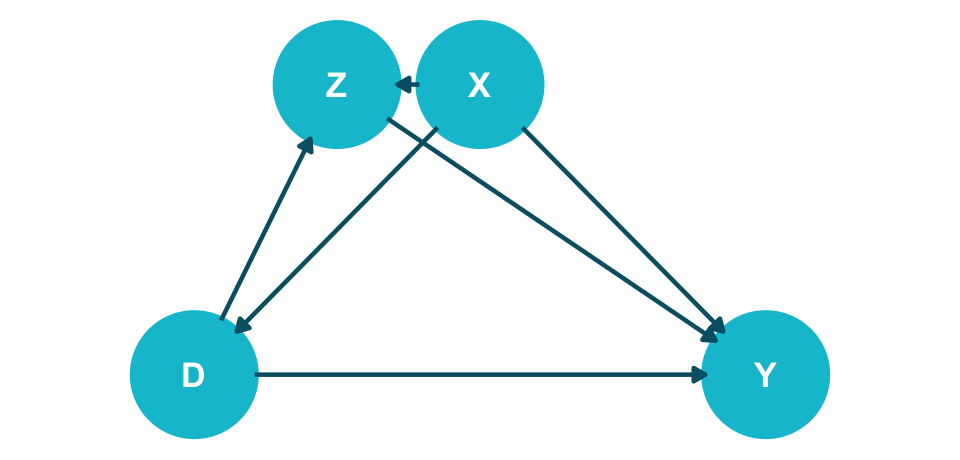
Rule: If \(Y \perp\!\!\!\perp_{G_{\overline{D},\, \underline{Z}}} Z \mid D, X\), then \(P(Y \mid do(D), do(Z), X) = P(Y \mid do(D), Z, X)\)

Check in \(G_{\overline{D},\, \underline{Z}}\) (delete into \(D\), out of \(Z\)): if confounding of \(Z\) on \(Y\) is blocked, replace \(do(Z)\) with observation.

Original graph \(G\):

\(\Rightarrow\)

\(G_{\overline{D},\, \underline{Z}}\) (delete into \(D\), out of \(Z\)):

\(Z \rightarrow Y\) deleted, arrows into \(D\) deleted. If \(X\) and \(D\) d-separate \(Z\) from \(Y\) in \(G_{\overline{D},\, \underline{Z}}\), then \(do(Z)\) can safely become observation of \(Z\). This is the workhorse rule that converts interventional quantities into observational ones.

Rule 2 is the most important. After deleting arrows out of Z (the do-operator on Z) and arrows into D (the do-operator on D), if Z is d-separated from Y given D and X, then intervening on Z is equivalent to merely observing Z. This is how do-calculus converts do-expressions into observational expressions; backdoor and frontdoor are special cases.

Rule 3: Irrelevant interventions can be dropped

Rule: If \(Y \perp\!\!\!\perp_{G_{\overline{D},\, \overline{Z(X)}}} Z \mid D, X\), then \(P(Y \mid do(D), do(Z), X) = P(Y \mid do(D), X)\)

Check in \(G_{\overline{D},\, \overline{Z}}\) (delete into \(D\), into \(Z\)): if \(Z\) cannot reach \(Y\), intervening on \(Z\) is pointless. \(Z(X)\): the subset of \(Z\) nodes that are not ancestors of any \(X\)-node in \(G_{\overline{D}}\).

Original graph \(G\):

\(\Rightarrow\)

\(G_{\overline{D},\, \overline{Z}}\) (delete into \(D\), into \(Z\)):

For all \(Z\) that are not ancestors of any \(X\) we condition on, we can delete all edges into \(Z\). If in \(G_{\overline{D},\, \overline{Z(X)}}\) the variable \(Z\) is (conditionally) independent of \(Y\), the do-operator for \(Z\) can be ignored.

Rule 3 handles the case where an intervention is simply irrelevant. After deleting arrows into both D and Z, if Z cannot reach Y given D and X, then do(Z) has no effect and can be dropped. The \(Z(X)\) restriction matters when Z is an ancestor of X: in that case we may not delete edges into Z, because conditioning on X can open backdoor paths between Z and Y that the surgery would falsely suppress.

The three rules of do-calculus — summary

Graph notation: \(G_{\overline{X}}\) = delete arrows into \(X\); \(G_{\underline{X}}\) = delete arrows out of \(X\).

Rule	Formal statement	Graphical condition	Plain English
R1	\(P(Y \mid do(D), Z, X) = P(Y \mid do(D), X)\)	\(Y \perp\!\!\!\perp_{G_{\overline{D}}} Z \mid D, X\)	Irrelevant observations can be dropped.
R2	\(P(Y \mid do(D), do(Z), X) = P(Y \mid do(D), Z, X)\)	\(Y \perp\!\!\!\perp_{G_{\overline{D},\, \underline{Z}}} Z \mid D, X\)	Intervention \(\rightarrow\) observation when confounding is blocked.
R3	\(P(Y \mid do(D), do(Z), X) = P(Y \mid do(D), X)\)	\(Y \perp\!\!\!\perp_{G_{\overline{D},\, \overline{Z(X)}}} Z \mid D, X\)	Irrelevant interventions can be dropped.

This summary table consolidates the three rules students just saw individually. Each rule corresponds to a specific graph modification and a d-separation check. Rule 1 handles observations, Rule 2 converts interventions to observations, Rule 3 drops interventions. Together they are complete: if a causal effect can be identified from observational data, these three rules will find the identifying expression. The table serves as a reference card students can return to.

Applying do-Calculus: the college wage premium

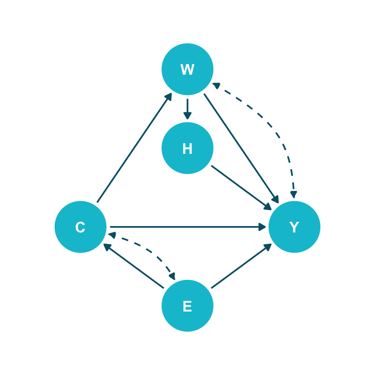
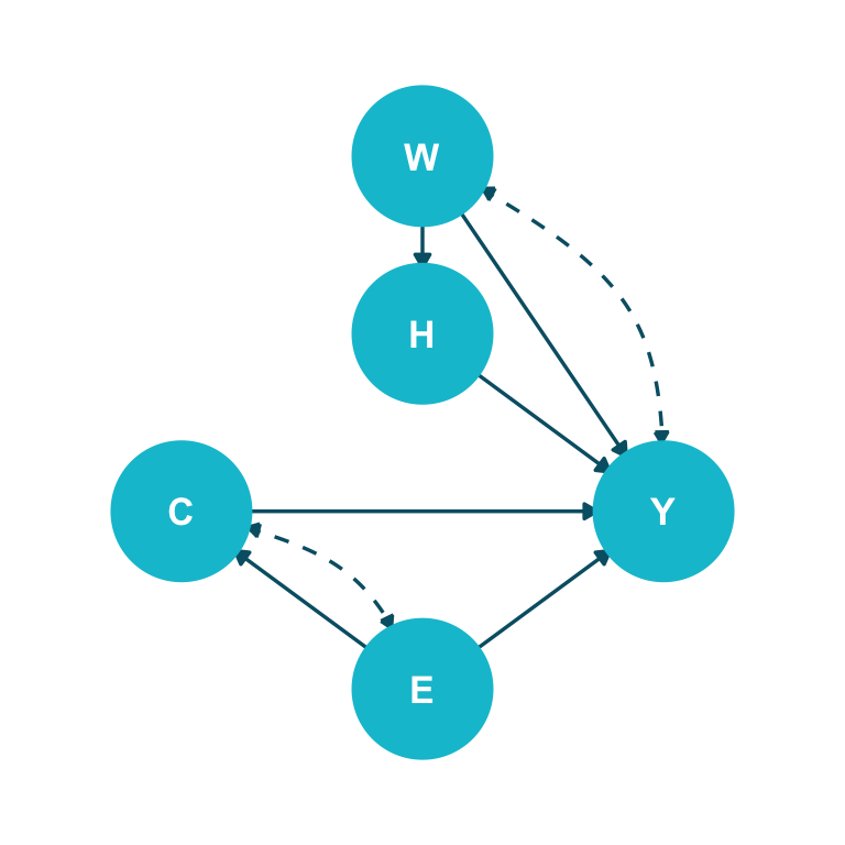
Stylized example of the college wage premium:

• \(C\): college degree
• \(Y\): earnings
• \(W\): occupation
• \(H\): work-related health
• \(E\): other socio-economic factors
• Dashed arrows: unobserved confounders

Task: Transform \(P(y \mid do(c))\) into a do-free expression by using the rules of do-calculus.

Causal Graph \(G\):

Step 1: Two backdoor paths in \(G\) can be blocked by \(E\). Conditioning and summing over all values of \(E\): \[P(y \mid do(c)) = \sum_{e} P(y \mid do(c), e)\, P(e \mid do(c))\]

The college wage premium is the canonical worked example for do-calculus: a richer DAG than the abstract Rule slides, with two unobserved-confounder edges (dashed \(Y \leftrightarrow W\) and \(C \leftrightarrow E\)). The task is to express \(P(y \mid do(c))\) as a do-free quantity. Step 1 is the law of total probability — marginalize over \(E\), which lies on the backdoor paths from \(C\) to \(Y\). Steps 2 and 3 follow on the next slide.

Applying do-Calculus: the college wage premium

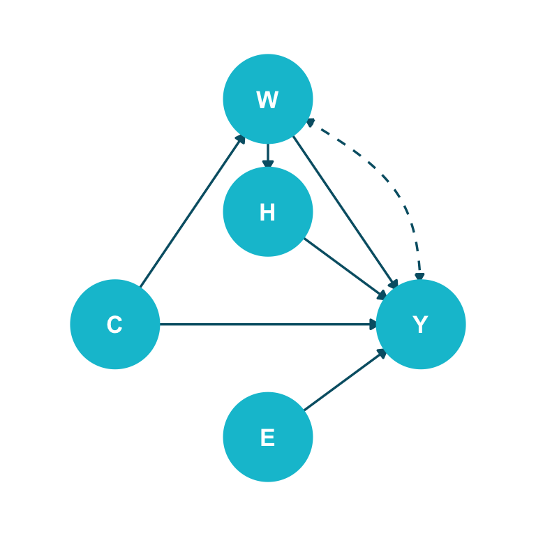
Step 2: Apply Rule 2 of do-calculus: \[P(y \mid do(c), e) = P(y \mid c, e) \quad\text{since}\quad Y \perp\!\!\!\perp_{G_{\underline{C}}} C \mid E\]

Manipulated Graph \(G_{\underline{C}}\):

Step 3: Apply Rule 3 of do-calculus: \[P(e \mid do(c)) = P(e) \quad\text{since}\quad E \perp\!\!\!\perp_{G_{\overline{C}}} C\]

Manipulated Graph \(G_{\overline{C}}\):

“Do-free” expression: \(P(y \mid do(c)) = \sum_{e} P(y \mid do(c), e)\,P(e \mid do(c)) = \sum_{e} P(y \mid c, e)\,P(e)\)

Step 2 applies Rule 2 in \(G_{\underline{C}}\) (arrows out of \(C\) deleted) to swap \(do(c)\) for observation of \(c\) — \(C\) and \(Y\) become d-separated given \(E\). Step 3 applies Rule 3 in \(G_{\overline{C}}\) (arrows into \(C\) deleted) to drop \(do(c)\) from the marginal of \(E\) — \(E\) becomes independent of \(C\). Substituting both into Step 1 collapses to a do-free identifying expression that depends only on observable conditional and marginal probabilities. The backdoor criterion is a theorem of do-calculus, not an independent result.

do-calculus is complete: if identification is possible, the rules find it

Completeness of do-Calculus (Huang & Valtorta 2006; Shpitser & Pearl 2006)

For any DAG \(G\) and any causal query \(P(Y \mid do(D))\):

• Either do-calculus can derive an identifying expression from observational distributions, or
• No such expression exists (the effect is not identifiable from observational data)

The three rules are all you need. Nothing is left on the table.

Practical implications:

• The ID algorithm (Shpitser and Pearl 2006) automates the application of do-calculus rules
• Software: causaleffect R package, dagitty, DoWhy (Python)
• You do not need to memorize or manually apply the three rules — software does it
• But understanding the logic helps you draw better DAGs and interpret the results

The completeness result is remarkable: three simple rules exhaust all possible identification strategies from observational data. Huang and Valtorta (2006) and Shpitser and Pearl (2006) independently proved this. The practical implication is twofold. First, software can automate identification completely — given a DAG, the ID algorithm either produces an identifying formula or proves none exists. Second, when the algorithm says the effect is not identifiable, this is not a limitation of the method but a fundamental limitation of the data. No estimator, no matter how sophisticated, can identify the effect without additional assumptions or data sources. This shifts the analyst’s effort from manual derivation to careful DAG construction, which is where domain expertise matters most.

Pearl’s Causal Hierarchy separates seeing, doing, and imagining

Layer	Name	Typical query	Notation	Example
L3	Counterfactual	“What would have happened?”	\(P(Y_d \mid D = d', Y = y')\)	Would this patient have survived under treatment, given they died without it?
L2	Intervention	“What happens if we act?”	\(P(Y \mid do(D = d))\)	What is the expected revenue if we set the ad budget to 100K?
L1	Association	“What do we observe?”	\(P(Y \mid D = d)\)	Customers who saw the ad bought more. Is the ad effective?

Causal Hierarchy Theorem (Bareinboim et al. 2022): Data at layer \(L_k\) cannot answer queries at layer \(L_{k+1}\) without additional assumptions or structure.

Pearl’s Causal Hierarchy, also called the Ladder of Causation, organizes all causal and statistical queries into three layers. Layer 1 is association: conditional probabilities, correlations, predictions. This is where standard statistics and machine learning operate. Layer 2 is intervention: what happens when we change something. This is where do-calculus and the adjustment formula live. Layer 3 is counterfactual: what would have happened to a specific individual under a different treatment, given what we observed. The Causal Hierarchy Theorem by Bareinboim et al. (2022) proves that data from a lower layer is, in general, insufficient to answer queries at a higher layer. This is a deep result. It means no amount of observational data can determine causal effects without assumptions, and no number of RCTs can determine individual counterfactuals without additional modeling. Session 01’s fundamental problem of causal inference is the L1 to L2 gap. The potential outcomes framework operates at L3.

Causal Discovery

Identification assumes the DAG. Where does the DAG come from?

Everything we have done so far — d-separation, the backdoor criterion, the frontdoor criterion, do-calculus — takes the DAG as a given input. The analyst draws the graph from domain knowledge, and the algorithms tell them which adjustments identify the causal effect. But this raises a deeper question: where does the DAG itself come from? Three honest answers exist. Domain experts draw it from substantive knowledge. Randomized experiments establish individual edges by intervention. And, when neither is available, causal discovery algorithms attempt to recover structure directly from observational data. This section is about that third option — its promise, its assumptions, and its honest limits.

DAGs are hypotheses, not data

A DAG encodes a causal hypothesis about how variables generate one another. It is the input to identification, not its output. Three sources fill that input:

Domain expertise

Subject-matter experts draw the graph from theory, mechanism, and prior studies. Strength: encodes substantive knowledge data alone cannot reveal. Weakness: experts disagree; biases creep in; some edges are simply unknown.

Experiments

A randomized intervention on \(D\) severs all incoming edges, isolating the effect \(D \to Y\). Strength: establishes individual edges by design. Weakness: expensive, slow, often infeasible (ethics, cost, scale).

Discovery from data

Algorithms search for graphs consistent with the observed conditional independencies (or the best-scoring fit). Strength: uses what we already have — observational data. Weakness: identifies a class of graphs, not always a unique one; assumption-heavy.

In practice, all three are combined: discovery proposes, expertise edits, experiments confirm.

DAGs are not data. They are hypotheses about a data-generating process. Three independent sources can produce them. Domain experts encode substantive knowledge — economists know wages depend on education and ability, doctors know infection precedes symptoms. This is essential and irreplaceable, but it is not infallible. Two experts often disagree about which edges exist, and certain mechanisms are simply outside any expert’s reach. Randomized experiments give the cleanest evidence for individual edges: a successful RCT on \(D \to Y\) establishes that edge by construction. But experiments are costly, slow, and frequently impossible. The third source — causal discovery from observational data — uses what we already have: large amounts of measured data. Discovery algorithms search for graphs that are consistent with the conditional independence structure observed in the data, or that score best under some fit criterion. The best practice combines all three: discovery generates candidate graphs, expert review prunes nonsensical structure, and where the stakes warrant, an experiment confirms a critical edge.

What can data alone tell us about the DAG?

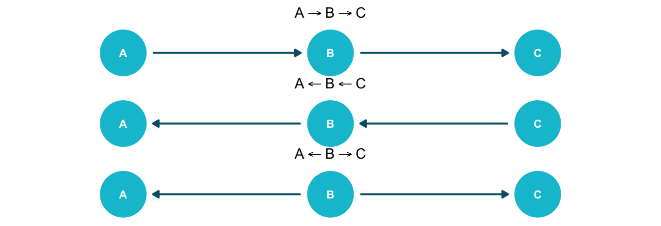
The Markov equivalence problem. Consider three DAGs over \(\{A, B, C\}\):

All three imply the same CI: \(A \perp\!\!\!\perp C \mid B\). Observational data cannot tell them apart.

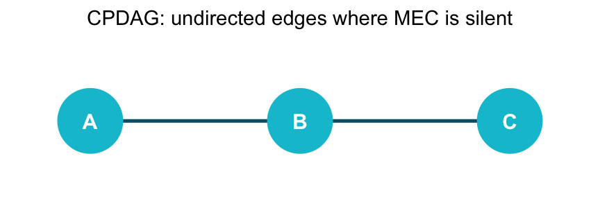
Markov equivalence class (MEC). DAGs that imply the same set of conditional independencies form an equivalence class. Discovery from observational data can recover the MEC — but no single member of it.

CPDAG (Completed Partially Directed Acyclic Graph) = the MEC’s graphical signature: directed edges where orientation is identified, undirected edges where it is not.

Punchline: discovery from observational data ⟹ a CPDAG, not a unique DAG. To go further, we need either an extra assumption (LiNGAM) or experimental data.

This is the central caveat of causal discovery, and the one students are most likely to misunderstand. Three different DAGs — the chain \(A \to B \to C\), the reverse chain \(A \leftarrow B \leftarrow C\), and the fork \(A \leftarrow B \to C\) — all imply exactly the same conditional independence: \(A\) and \(C\) are independent given \(B\). They are Markov equivalent. No statistical test on observational data can distinguish among them. The fork (a confounder) and the two chains (mediation in either direction) make the same predictions about every conditional probability. The collider \(A \to B \leftarrow C\) is the exception — it implies \(A \perp\!\!\!\perp C\) marginally but \(A \not\perp\!\!\!\perp C \mid B\), which is detectable from data and breaks the equivalence class. So observational discovery returns a Markov equivalence class, summarized graphically as a CPDAG: a partially directed graph where some edges are directed (where v-structures and Meek’s rules pin them down) and others remain undirected. The undirected edges are the genuine ambiguity — three different causal stories that the data simply cannot adjudicate. To go further we need either an additional assumption (LiNGAM uses non-Gaussianity), structural restrictions (additive noise models), or experimental data.

Three families of causal-discovery algorithms

Family	Central question	Output	Key assumption	Examples
Constraint-based	Which conditional independencies hold in the data?	CPDAG (or PAG with latents)	Faithfulness	PC, FCI
Score-based	Which DAG fits the data best under a score (BIC, BDe)?	CPDAG	Score consistency	GES, GIES
Functional / non-Gaussian	Can asymmetries in the noise distribution break the MEC tie?	Unique DAG	Linearity + non-Gaussian noise (or nonlinearity)	LiNGAM, ANM

We will walk PC in detail (the canonical example), then sketch GES and LiNGAM at conceptual depth.

The discovery literature is large but organizes naturally into three families, each defined by what it uses in the data to recover structure. Constraint-based methods — most famously the PC algorithm by Spirtes, Glymour, and Scheines (2000) — read off the graph from a sequence of conditional independence tests. Their central commitment is faithfulness: the assumption that every CI in the distribution corresponds to a d-separation in the graph and vice versa. Score-based methods take a different tack: they define a global goodness-of-fit score (typically BIC for Gaussian or BDe for discrete data), then search the space of DAGs for the highest-scoring one. GES, by Chickering (2002), is the canonical example. Constraint and score methods both return a CPDAG — they cannot distinguish among Markov-equivalent graphs. The third family breaks that tie by adding a structural assumption beyond CIs. LiNGAM, by Shimizu et al. (2006), assumes the data come from a linear SEM with non-Gaussian noise; under this assumption, the unique DAG is identifiable from the data, not just the equivalence class. Additive noise models (ANM) generalize this to nonlinear functions with additive noise. We walk PC in full detail because it is the most-taught and most-implemented; the others get one or two slides each at conceptual depth — enough that students can read the literature and recognize the methods in software.

PC algorithm: discover the skeleton, then orient

PC (Spirtes, Glymour, and Scheines 2000) turns the d-separation criterion backwards: starting from “everything is connected”, remove edges as conditional independencies are detected, then orient as far as the data allows.

Phase 1 — Skeleton

Begin with the complete undirected graph. For each edge \(X - Y\), search for a separating set \(S\) such that \(X \perp\!\!\!\perp Y \mid S\). If one exists, delete the edge and record \(S\) as the separating set. Increase \(|S|\) from \(0, 1, 2, \dots\) until no edges remain to test.

Phase 2 — V-structures

For each unshielded triple \(X - Z - Y\) (i.e., \(X\) and \(Y\) are not adjacent), check the recorded separating set: if \(Z \notin S\), orient as \(X \to Z \leftarrow Y\) (a collider).

Phase 3 — Meek’s rules

Propagate orientations using four logical rules (R1–R4): never create a new v-structure or a directed cycle. Anything left undirected is genuinely ambiguous under the data alone.

Output: a CPDAG representing the Markov equivalence class.

PC is the canonical constraint-based discovery algorithm and the easiest to explain because each phase corresponds to a clean idea. Phase 1 — skeleton search — exploits the fact that an edge \(X - Y\) in a DAG cannot be d-separated by any set: directly adjacent variables remain dependent in every conditioning scenario. So the contrapositive lets us delete an edge as soon as we find a single set \(S\) that makes them conditionally independent. The algorithm searches over conditioning sets in increasing size: first marginal independence (\(|S| = 0\)), then \(|S| = 1\), and so on. Recording the separating set \(S\) for each removed edge is critical for Phase 2. Phase 2 — v-structure orientation — uses the asymmetry of colliders. In an unshielded triple \(X - Z - Y\) where \(X\) and \(Y\) are not adjacent, \(Z\) is either a collider (\(X \to Z \leftarrow Y\)) or part of a chain/fork. The collider case is the only one where \(Z\) is not in the separating set that made \(X\) and \(Y\) independent. So if we recorded \(S\) from Phase 1 and \(Z \notin S\), we can orient the triple as a collider. Phase 3 — Meek’s rules — propagates these orientations conservatively: any new orientation forced to avoid (a) creating a new v-structure that wasn’t detected in Phase 2, or (b) creating a directed cycle. The four rules R1–R4 are these forced orientations applied iteratively until nothing more can be inferred. What remains undirected at the end is genuinely ambiguous: the data is consistent with either direction. The output is a CPDAG: directed where the data identifies orientation, undirected where Markov equivalence prevents identification.

Toy run: 5-node example with one isolated node

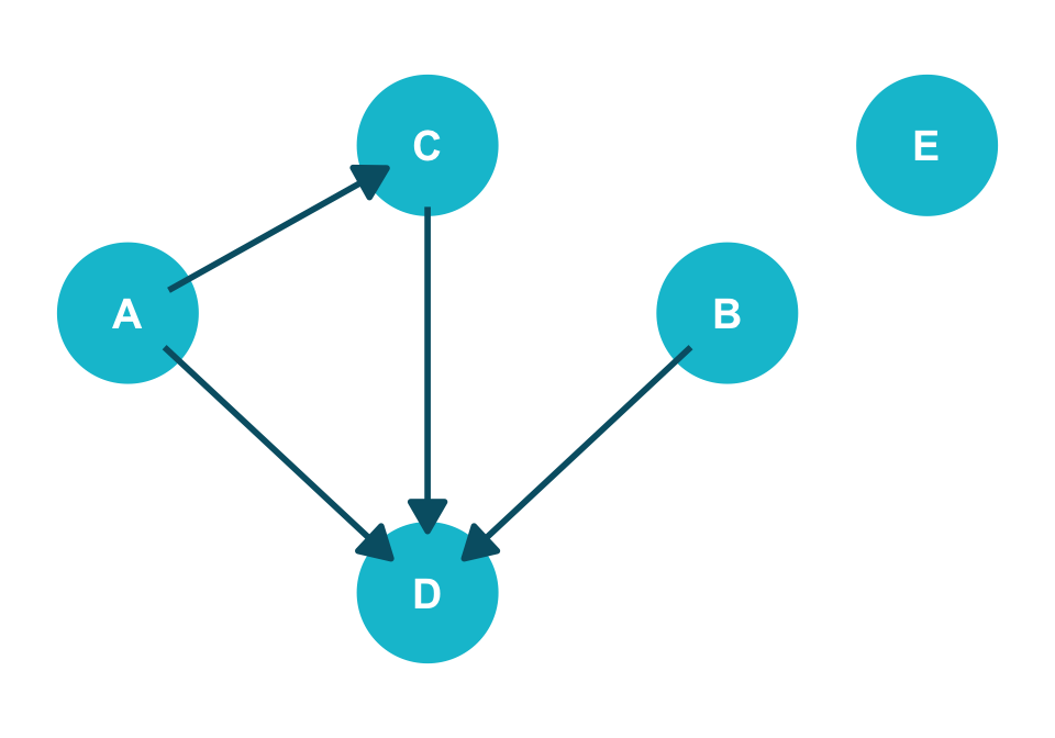
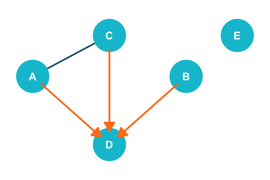
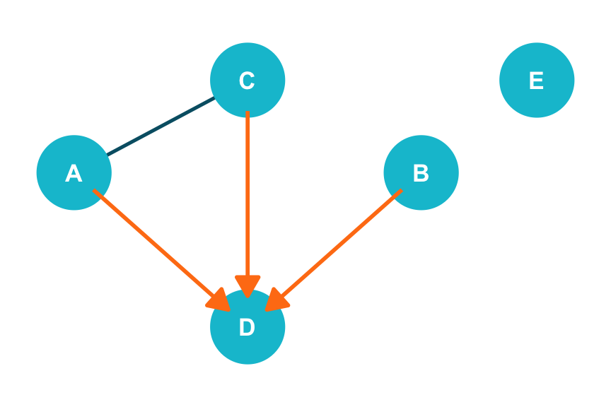
Ground truth: \(A \to C\), \(A \to D\), \(B \to D\), \(C \to D\). \(D\) is a 3-parent collider; \(E\) is isolated.

Conditional independencies implied by the DAG:

From d-separation

• \(E \perp\!\!\!\perp \{A, B, C, D\}\) marginally — no edges
• \(A \perp\!\!\!\perp B\) marginally — only paths via collider \(D\)
• \(B \perp\!\!\!\perp C\) marginally — only path \(B \to D \leftarrow C\) blocked
• \(A \not\perp\!\!\!\perp B \mid D\) — conditioning on collider opens path
• \(A\) and \(C\): directly adjacent, never independent

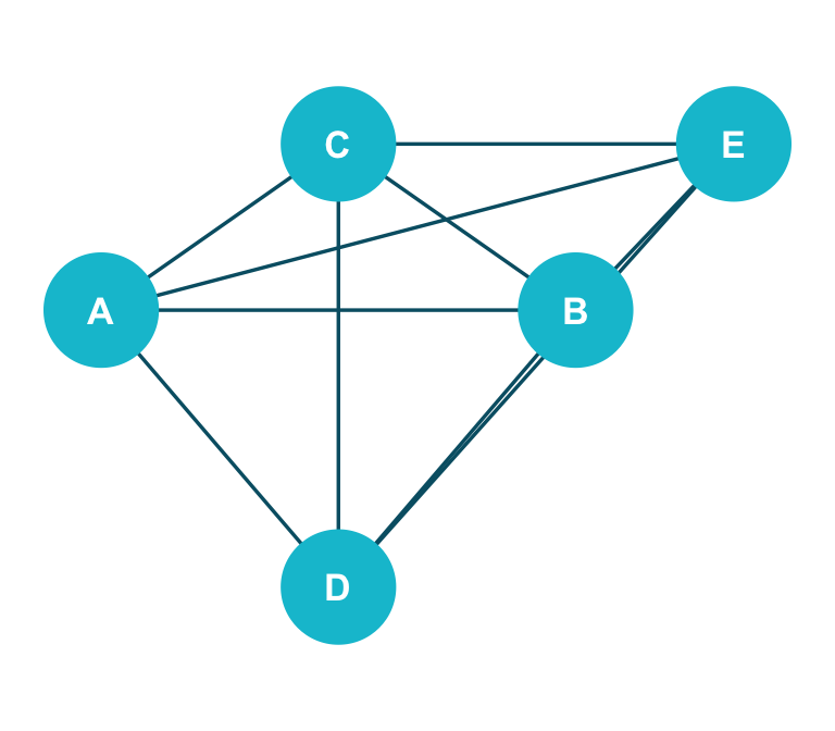
Goal of PC: start from \(K_5\) (10 edges), use these CIs (read from data) to recover the CPDAG. Then check: how close to ground truth?

This toy example is the canonical PC-walkthrough DAG from the 2022 lecture deck. The true graph has four causal edges — \(A \to C\), \(A \to D\), \(B \to D\), \(C \to D\) — making \(D\) a collider with three parents. Node \(E\) has no edges to any other variable: it is a pure decoy whose role is to demonstrate that PC correctly identifies and discards fully-disconnected variables during the marginal-independence sweep. The implied conditional independencies are the signal that PC will read from the data. \(E\) is marginally independent of every other node because no path exists. \(A\) and \(B\) are marginally independent because the only paths between them, \(A \to D \leftarrow B\) and \(A \to C \to D \leftarrow B\), are both blocked at the collider \(D\). Similarly \(B\) and \(C\) are marginally independent because the path \(B \to D \leftarrow C\) is collider-blocked. Crucially, conditioning on \(D\) opens the collider, so \(A \not\perp\!\!\!\perp B \mid D\) — this signature is what PC will use later to orient \(D\) as a collider. \(A\) and \(C\) are directly adjacent so they are never independent under any conditioning set. PC begins with the complete graph \(K_5\) on \(\{A, B, C, D, E\}\) — ten edges — and removes edges as it finds conditional independencies. The next slides walk through that removal step by step.

PC step 1: skeleton phase removes edges by CI tests

Start: complete \(K_5\) (10 edges)

\(\Rightarrow\)

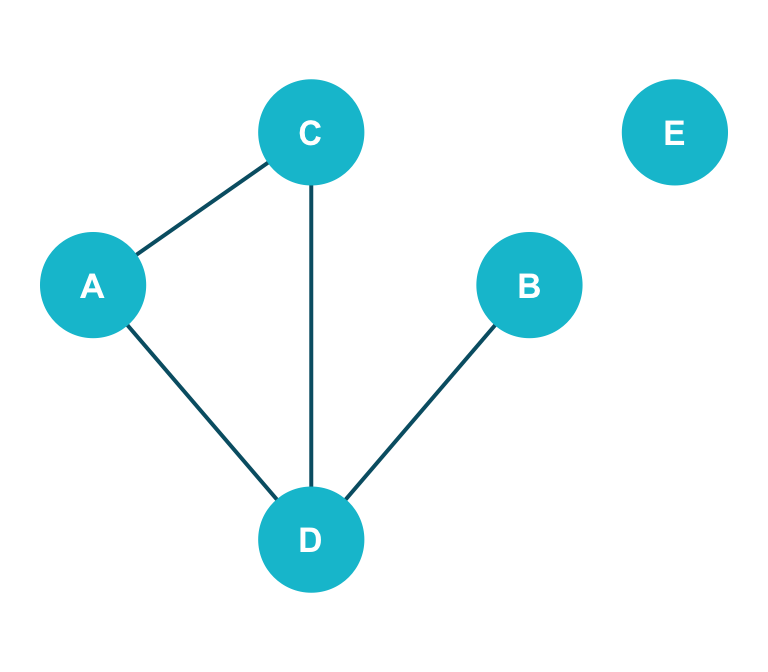
\(|S| = 0\): drop 6 edges (4 to \(E\) + \(A\!-\!B\) + \(B\!-\!C\))

Final skeleton (4 edges)

All separating sets are \(\varnothing\). \(|S|\!=\!1, 2\) remove no further edges.

The skeleton phase begins with the complete undirected graph \(K_5\) on five nodes — ten edges in total. PC then tests conditional independence with conditioning set sizes \(|S| = 0, 1, 2, \ldots\), removing an edge whenever a CI test succeeds. At \(|S| = 0\) (marginal independence) the algorithm finds six successful tests in our example. The four edges incident to \(E\) all drop because \(E\) is marginally independent of every other variable — a pure decoy with no causal connections. The edge \(A - B\) drops because the only paths connecting \(A\) and \(B\) in the true DAG, \(A \to D \leftarrow B\) and \(A \to C \to D \leftarrow B\), both pass through the collider \(D\), which blocks them under the empty conditioning set. Similarly \(B - C\) drops because the only path \(B \to D \leftarrow C\) is collider-blocked. After this single sweep, only four edges remain: \(A - C\), \(A - D\), \(B - D\), \(C - D\) — the four genuine adjacencies in the ground-truth DAG. At \(|S| = 1\) and \(|S| = 2\), no further conditional independencies can be found among these four edges (they are all true adjacencies, never independent under any conditioning set), so the skeleton phase terminates. The crucial bookkeeping detail: PC records the separating set used for each removal — all \(\varnothing\) in this example. These separating sets are the input to the v-structure phase that follows. In the rendered figure, orange highlights the four surviving edges; PC has pruned the search space from ten potential edges down to four real ones using only marginal CIs.

PC step 2: orient v-structures from separating sets

Test every unshielded triple \(X - Z - Y\) (\(X, Y\) not adjacent):

Rule

If \(Z \notin \text{sep}(X, Y)\), orient \(X \to Z \leftarrow Y\) (collider). Else, leave undirected.

Apply to our triples

Skeleton has two unshielded triples sharing \(D\):

• Pair \(\{A, B\}\), neighbor \(D\): \(D \notin \text{sep}(A, B) = \varnothing\) → collider! Orient \(A \to D \leftarrow B\).
• Pair \(\{B, C\}\), neighbor \(D\): \(D \notin \text{sep}(B, C) = \varnothing\) → collider! Orient \(B \to D \leftarrow C\).
• Pair \(\{A, B\}\), neighbor \(C\): \(C\) is not adjacent to \(B\) — not a triple.

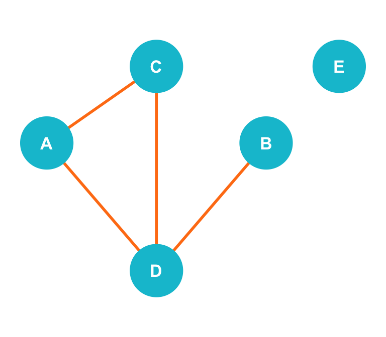
Three arrows oriented at the collider \(D\) — \(A \to D\), \(B \to D\), \(C \to D\).

(Edge \(A - C\) remains undirected — no v-structure involves it.)

The v-structure phase looks at every triple where two non-adjacent nodes share a common neighbor. The collider rule is: orient as \(X \to Z \leftarrow Y\) if and only if \(Z\) is not in the separating set used to remove the edge \(X - Y\) in the skeleton phase. The intuition: in a true v-structure, conditioning on the collider opens a path between \(X\) and \(Y\) — so the separating set that made them independent could not have included the collider. Contrapositive: if \(Z\) is in the separating set, the triple is a chain or a fork, not a collider, and we leave it undirected. In our skeleton, the non-adjacent pairs are \(\{A, B\}\) and \(\{B, C\}\), both with separating set \(\varnothing\) (they were marginally independent in the skeleton phase). Each pair has \(D\) as a common neighbor, and \(D\) is not in \(\varnothing\) — so PC orients both as v-structures. The result is three arrowheads pointing into \(D\): \(A \to D\), \(B \to D\), \(C \to D\). This matches the ground truth exactly: \(D\) has three parents in the true DAG. The edge \(A - C\) remains undirected because no unshielded triple involves it as a middle node — \(A\) and \(C\) are the endpoints of one triple (\(A - C - D\), but \(A\) and \(D\) are adjacent so it’s shielded, not unshielded), never the middle. PC has correctly identified that \(D\) is a 3-parent collider from observational data alone, and has done so by reading the marginal independencies \(A \perp\!\!\!\perp B\) and \(B \perp\!\!\!\perp C\) together with their respective common neighbor \(D\). The single remaining undirected edge \(A - C\) will be handled — or not — by Meek’s rules in the next step.

PC step 3: Meek’s rules propagate orientations

Four rules, applied iteratively:

R1: avoid new v-structures

If \(X \to Z - Y\) and \(X, Y\) not adjacent, then orient \(Z \to Y\) (otherwise \(X \to Z \leftarrow Y\) would be a v-structure we did not detect).

R2: avoid cycles

If \(X \to Z \to Y\) and \(X - Y\), then orient \(X \to Y\).

R3, R4 (continued)

R3 and R4 handle further propagation cases, all rooted in the same two principles: no new v-structures, no directed cycles.

In our toy DAG: v-structures already pinned \(A \to D\), \(B \to D\), \(C \to D\). R1 needs an outgoing oriented edge feeding an undirected neighbor — but every oriented arrow points into \(D\), which has no undirected edges leaving it. \(A - C\) stays undirected.

PC’s output: CPDAG

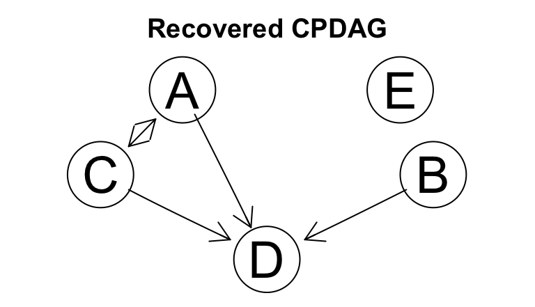
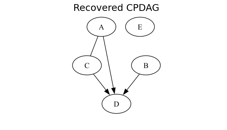
Ground-truth DAG: \(A \to C\), \(A \to D\), \(B \to D\), \(C \to D\). PC recovered the skeleton, the collider \(D\) (3 oriented arrows), and isolated \(E\). \(A - C\) stays undirected — equivalence-class undetermined.

Meek’s four rules complete the orientation phase by propagating the v-structure information conservatively. Rule R1 (avoid new v-structures): if we have \(X \to Z - Y\) where \(X\) and \(Y\) are not adjacent, we must orient \(Z \to Y\), because the alternative \(Z \leftarrow Y\) would create a new v-structure \(X \to Z \leftarrow Y\) that we would have detected in Phase 2 had it existed. Rule R2 (avoid cycles): if we have a directed path \(X \to Z \to Y\) and an undirected edge \(X - Y\), we must orient \(X \to Y\) to avoid the cycle. Rules R3 and R4 handle compound cases. In our toy example, the v-structure phase pinned three arrows pointing into the collider \(D\). R1 needs the oriented arrow to point outward from a node \(Z\) that also has an undirected neighbor — but every oriented arrow in our graph points into \(D\), and \(D\) has no undirected outgoing edges. R2 would require a directed two-step path, which we don’t have. So Meek’s rules do not propagate further. The final CPDAG keeps \(A - C\) undirected. The remaining undirected edge is equivalence-class undetermined: the ground-truth orientation \(A \to C\) is observationally indistinguishable from \(A \leftarrow C\), because both alternative DAGs imply the same conditional independencies and avoid creating any new v-structure. This is a critical pedagogical moment: PC is not failing — observational data fundamentally cannot adjudicate between Markov-equivalent DAGs. The equivalence class containing the ground truth is the most that PC can return. Notice also that PC has correctly identified \(E\) as a fully-disconnected node by dropping all its edges in the marginal independence sweep — this is the algorithm’s robustness to “decoy” variables in real data.

PC’s assumptions and how they fail

Assumption	What it buys us	How it fails	Symptom
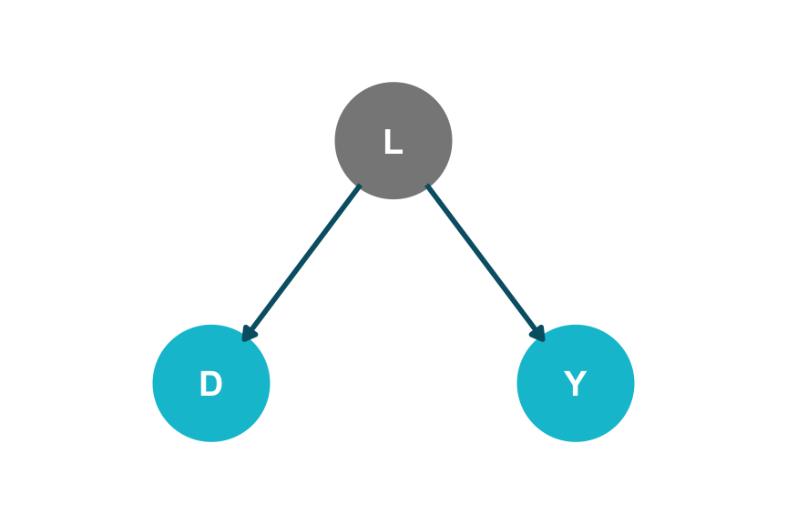
Causal sufficiency	No latent confounders — every common cause is observed.	Hidden variable \(L\) confounds \(D, Y\).	Spurious direct edge \(D - Y\) that should be a fork.
Faithfulness	Every CI in the data corresponds to a d-separation in the DAG.	Two paths exactly cancel (positive direct + negative indirect).	Edge wrongly removed → wrong skeleton.
Correct CI test	Test detects the right CIs at finite sample size.	Wrong family (Gaussian test on non-linear data); too small \(n\).	Random edges added or removed; output unstable.
No selection bias	Sample is not implicitly conditioned on a collider.	Survivor data; cohort filtering on outcome.	Spurious dependencies between independent causes.

Causal sufficiency is the heaviest. We address it next with FCI.

PC has four major assumptions, each of which can fail in practice. Causal sufficiency — that all common causes of measured variables are themselves measured — is by far the most often violated. In any real dataset, latent confounders are the rule, not the exception. When they exist, PC mistakes a confounder-induced dependency for a direct edge. Faithfulness is more subtle: it says the DAG and the observed CI structure are in one-to-one correspondence. It can fail when two paths between \(X\) and \(Y\) cancel exactly — for instance, a positive direct effect \(X \to Y\) that is exactly offset by a negative indirect effect through a mediator. Such cancellations are rare in continuous parameters (zero Lebesgue measure) but can be exact under deterministic constraints or in fine-tuned simulations. The CI test choice is a finite-sample issue: PC presumes a test that detects the correct CIs at the available sample size. Gaussian partial-correlation tests work well for linear-Gaussian data, but applying them to nonlinear or heavy-tailed data produces unreliable removals. Selection bias — when the sample itself is conditioned on a collider — induces spurious dependencies that PC reads as edges. Cohort studies that filter on outcome status are a classic example. Of the four, causal sufficiency is the one that triggered an entire algorithmic response: the FCI algorithm extends PC to the latent-confounder case by augmenting the output graph with bidirected edges and partial directionality marks. We meet it next.

What if causal sufficiency fails? FCI extends PC

Setup. A latent \(L\) confounds \(D\) and \(Y\); \(L\) is unobserved.

PC sees only \(D\) and \(Y\). They are dependent (because of \(L\)), so PC connects them with a direct edge \(D - Y\). Wrong: there is no direct effect.

FCI (Spirtes, Meek, and Richardson 1995) outputs a PAG (Partial Ancestral Graph) with richer edge marks:

PAG edge marks

• \(D \to Y\): \(D\) causes \(Y\) (direct or via observed mediators).
• \(D \leftrightarrow Y\): \(D\) and \(Y\) share an unmeasured common cause.
• \(D \;\circ\!\!\to\; Y\): \(Y\) is not a cause of \(D\), but the rest is unidentified.
• \(D \;\circ\!\!-\!\!\circ\; Y\): orientation completely unidentified.

In our setup FCI returns \(D \leftrightarrow Y\) — the bidirected mark flags the latent confounder instead of mistaking it for a direct edge.

FCI’s price: a richer output that is harder to read, more CI tests, and more orientation rules.

FCI — the Fast Causal Inference algorithm by Spirtes, Meek, and Richardson (1995) — extends PC to the case where causal sufficiency fails. The setup is the simplest possible illustration: a latent variable \(L\) that we do not observe is the common cause of \(D\) and \(Y\). PC, which sees only \(\{D, Y\}\), finds that they are dependent and concludes there must be a direct edge between them. This is wrong — there is no direct causal effect; the entire dependency is induced by the unmeasured confounder. FCI’s response is to augment the output graph with new edge marks. Instead of just directed and undirected edges, a PAG has four kinds of marks at each end of an edge: an arrowhead, a tail, a circle (meaning “unidentified”), and the absence of an edge. Combinations give five edge types: \(\to\), \(\leftrightarrow\), \(\circ\!\to\), \(\circ\!-\!\circ\), and the regular undirected \(-\). The bidirected \(\leftrightarrow\) explicitly says “the data implies an unmeasured common cause” without forcing a direct edge that does not exist. The cost is that FCI’s CI-test schedule is longer than PC’s (it must check separating sets that include latents in principle), and the orientation rule set is larger. But for any real-world dataset where you suspect latent confounders — which is essentially every dataset — FCI is the tool to reach for, not PC.

GES: search the space of DAGs by score

GES (Chickering 2002) takes a different route to the same destination. Instead of asking “which CIs hold?”, it asks “which DAG scores best?” — and walks through DAG space greedily.

Score function (BIC for Gaussian data):

\[\text{BIC}(G; \text{data}) = -2 \log L(G) + k(G) \log n\]

• \(\log L(G)\): log-likelihood of the data given graph \(G\).
• \(k(G)\): number of parameters (edges + variances).
• \(\log n\): complexity penalty — punishes overly dense graphs.

Two-phase greedy search:

Forward phase

Start from the empty graph. At each step, add the single edge that improves BIC the most. Stop when no edge addition improves the score.

Backward phase

From the forward-phase output, remove the single edge that improves BIC the most. Stop when no removal improves the score.

Output: a CPDAG — same equivalence-class limit as PC, by a different route.

GES — Greedy Equivalence Search by Chickering (2002) — is the canonical score-based discovery algorithm. The score function is typically the Bayesian Information Criterion: BIC equals minus-twice the log-likelihood plus a penalty term that grows with the number of parameters and the log of the sample size. Maximizing log-likelihood alone would always favor the densest graph (every edge added improves fit), so the BIC penalty is what makes the search well-posed: at some point, adding an edge no longer pays for the parameter complexity it introduces. GES walks DAG space in two phases. The forward phase starts from the empty graph and adds the single edge that most improves BIC, repeating until no addition improves the score. The backward phase then removes the single edge whose removal most improves BIC, repeating until no removal helps. The two-phase structure has a clean theoretical guarantee: under standard regularity conditions, GES converges to the true CPDAG as \(n \to \infty\). So GES and PC, as \(n \to \infty\), identify the same object — the Markov equivalence class — by completely different routes. PC chains together a thousand small statistical decisions; GES makes one global optimization decision. The two routes have different finite-sample behavior, which we contrast next.

GES vs. PC: same destination, different vehicle

Property	PC (constraint)	GES (score)
Asymptotic limit	CPDAG (Markov equivalence class)	CPDAG (same)
Per-step decision	Many local CI tests (each edge has its own test).	One global score, evaluated under each candidate edit.
Small-sample stability	Sensitive: a single noisy CI test propagates into wrong skeleton.	More stable: BIC integrates over all data at once.
High-dim scaling	Better: tests are fast; can prune many edges quickly.	Worse: each candidate evaluation requires a likelihood fit.
What can go wrong	Faithfulness violations; bad CI test family.	Wrong likelihood model (e.g., Gaussian on heavy tails).

In practice: run both when sample size permits, and check whether they agree. Disagreement is informative.

PC and GES converge to the same object asymptotically — the CPDAG of the data-generating distribution — but they differ substantially in finite-sample behavior. PC’s per-step decision is a local CI test. Each test contributes its own Type I and Type II errors, and a single false negative early in the skeleton phase can propagate into a wrong CPDAG that no later step recovers. GES, by contrast, makes one global decision per step: which single edge edit improves a model-wide score the most. This integrates information across the entire dataset and tends to be more stable in small samples. The flip side is computational cost: GES must fit a likelihood for every candidate edge edit, and that scales worse than PC’s local CI tests on high-dimensional data. The failure modes also differ. PC’s enemy is faithfulness violations (CI tests that detect the wrong CIs because of cancellations) and bad CI test choice. GES’s enemy is a misspecified likelihood — using Gaussian BIC on heavy-tailed or nonlinear data gives a score that does not reflect the true generating mechanism. The practical advice in any moderate-sample-size setting: run both and check agreement. When they agree, you have a more robust answer than either alone. When they disagree, that disagreement is itself informative — it points at exactly where the assumptions diverge.

LiNGAM: non-Gaussian noise breaks the equivalence class

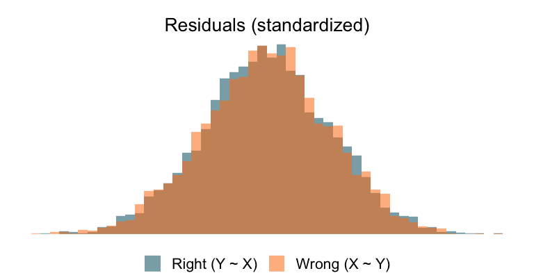
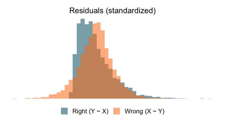
True model \(Y = \beta X + \varepsilon_Y\), \(\varepsilon_Y \perp X\). Right \(Y \sim X\): residuals \(\hat\varepsilon \approx \varepsilon_Y\) (= noise). Wrong \(X \sim Y\): residuals \(\hat\varepsilon^* = X - \hat\gamma Y\) keep a remnant of \(X\) — OLS only forces them uncorrelated with \(Y\), not independent.

Gaussian noise — residual shapes match

Both bells coincide. The remnant is there algebraically, but Gaussians are closed under linear combinations — every shape statistic looks identical. Direction unidentifiable.

Non-Gaussian noise (gamma) — shapes diverge

Right residuals = the skewed noise. Wrong residuals \(\propto X - \varepsilon_Y\) are symmetric (two skews with opposite signs cancel asymmetry). Direction identifiable.

LiNGAM (via ICA) listens for the gap between right- and wrong-direction residuals. Gaussianity hides it; non-Gaussianity exposes it. (Shimizu et al. 2006)

The two histograms on each side are regression residuals, not the raw noise. The pedagogical point is the relation between residuals and noise under the two regression directions. In the right direction (\(Y \sim X\), the data-generating direction), the residuals \(\hat\varepsilon = Y - \hat\beta X\) are an unbiased estimate of the noise \(\varepsilon_Y\) itself, so their distribution converges to the noise distribution. In the wrong direction (\(X \sim Y\), the reversed regression), the residuals \(\hat\varepsilon^* = X - \hat\gamma Y\) are not an estimate of any noise term that exists in the true model — they are a linear combination \(\hat\varepsilon^* \propto X - \varepsilon_Y\) of the cause variable and the original noise. OLS forces this combination to be uncorrelated with \(Y\), but it cannot force independence. So the residual carries information about the regressor even after the regression is run.

When the noise is Gaussian, this information is invisible to any second-order statistic, because Gaussians are closed under arbitrary linear combinations and rotations — both the right-direction and wrong-direction residuals end up Gaussian, and after standardizing they have the same shape, the same kurtosis, the same everything that any test could measure. The right and wrong models leave the same observational fingerprint. This is the precise sense in which \(X \to Y\) and \(Y \to X\) are Markov-equivalent under Gaussianity.

When the noise is non-Gaussian — here, gamma-distributed and right-skewed — the picture flips. Right-direction residuals stay skewed (they are the noise, up to sampling error). Wrong-direction residuals become symmetric: a difference of two i.i.d. skewed variables is symmetric, even though each variable individually is not. The two histograms now have visibly different shapes — one skewed, one symmetric — and any independence test sensitive to higher moments will reject independence between \(\hat\varepsilon^*\) and \(Y\). LiNGAM operationalizes this with Independent Component Analysis: ICA finds the linear un-mixing of the variables that makes the recovered components maximally non-Gaussian and mutually independent. That un-mixing is unique only when at most one true noise source is Gaussian. The recovered un-mixing matrix, after the right permutation, is lower-triangular, which fixes the causal ordering — and therefore the unique DAG, not just the Markov-equivalence class. The price is the structural assumption (linearity + non-Gaussian noise); the gain is identifiability beyond what PC or GES can ever deliver.

How LiNGAM works: ICA on the residuals

The model assumption: \(\mathbf{x} = B\mathbf{x} + \mathbf{e}\), where \(B\) is a strictly lower-triangular matrix (after permutation) and the noise \(\mathbf{e}\) has independent, non-Gaussian components.

Step 1 — Solve for the noise

Rearrange: \(\mathbf{e} = (I - B)\mathbf{x} = A\mathbf{x}\). The matrix \(A\) “un-mixes” the variables back into independent noise sources.

Step 2 — ICA

Independent Component Analysis recovers the un-mixing matrix \(A\) (up to permutation and scaling) by maximizing non-Gaussianity of the recovered components. This is the step that fails for Gaussian noise — Gaussians are rotationally symmetric, so ICA cannot pin down rotation.

Step 3 — Permute and scale

Permute the rows of \(A\) to make the diagonal as close to 1 as possible. The permutation that succeeds gives the causal ordering: variables earlier in the ordering cause variables later. Read off \(B = I - A\) to get edge weights.

Output: a unique DAG with estimated edge weights — assuming linearity and at most one Gaussian noise component hold.

The LiNGAM algorithm proceeds in three steps. Step 1 inverts the SEM. The structural model says each variable is a linear function of its parents plus an independent noise term: \(\mathbf{x} = B\mathbf{x} + \mathbf{e}\), where \(B\) has zeros on the diagonal and is strictly lower-triangular under the true causal ordering. Solving for \(\mathbf{e}\) gives \(\mathbf{e} = (I - B)\mathbf{x}\), and we call \(A = (I - B)\) the un-mixing matrix. Step 2 recovers \(A\) from data using Independent Component Analysis. ICA exploits the fact that under the model, the noise components are mutually independent and non-Gaussian. ICA looks for the linear transformation of the observed data that maximizes non-Gaussianity in each output component — the resulting components must be the original noise sources, up to permutation and rescaling. This is the step where the algorithm fundamentally requires non-Gaussianity: Gaussians are closed under arbitrary rotations, so ICA cannot distinguish between different rotational mixings of Gaussian sources. Step 3 reverses the permutation indeterminacy. We need to find the row permutation of \(A\) that makes its diagonal entries as close to 1 as possible — this corresponds to the unique permutation that places it in lower-triangular form when written as \(A = I - B\). The permutation that succeeds gives the causal ordering: variable index 1 is the source, index 2 is caused only by variable 1, and so on. Reading off \(B = I - A\) then gives the directed edges and their weights. The total cost of going from MEC to unique DAG is one structural assumption: linearity with non-Gaussian noise. ANM (Additive Noise Models, Hoyer et al. 2008) generalizes the same idea to nonlinear functions, replacing the linearity assumption with the much weaker requirement that the noise enters additively.

Hands-on: discover a DAG from simulated data

Same 5-node toy from the walkthrough — ground truth \(A \to C\), \(A \to D\), \(B \to D\), \(C \to D\), with \(E\) isolated. Simulate \(n = 500\), run PC, and read the recovered CPDAG.

• R
• Python

suppressPackageStartupMessages({
  library(pcalg)
  library(Rgraphviz)
})

set.seed(1); n <- 500
A <- rnorm(n); B <- rnorm(n); E <- rnorm(n)
C <- 0.7 * A + rnorm(n)
D <- 0.6 * A + 0.6 * B + 0.5 * C + rnorm(n)

dat <- data.frame(A = A, B = B, C = C, D = D, E = E)

fit <- pc(suffStat = list(C = cor(dat), n = nrow(dat)),
          indepTest = gaussCItest,
          alpha = 0.05,
          labels = colnames(dat))

plot(fit, main = "Recovered CPDAG")

import io
import numpy as np
import matplotlib.pyplot as plt
from PIL import Image
from causallearn.search.ConstraintBased.PC import pc
from causallearn.utils.GraphUtils import GraphUtils

np.random.seed(1); n = 500
A = np.random.randn(n); B = np.random.randn(n); E = np.random.randn(n)
C = 0.7 * A + np.random.randn(n)
D = 0.6 * A + 0.6 * B + 0.5 * C + np.random.randn(n)

data = np.column_stack([A, B, C, D, E])

cg = pc(data, alpha=0.05, indep_test='fisherz', show_progress=False)

pyd = GraphUtils.to_pydot(cg.G, labels=['A', 'B', 'C', 'D', 'E'])
img = Image.open(io.BytesIO(pyd.create_png()))
fig, ax = plt.subplots(figsize=(4, 2.3))
_ = ax.imshow(img)
_ = ax.set_title('Recovered CPDAG')
ax.set_axis_off()

This slide closes the loop on the hand-walked example. The simulated SEM matches the toy run exactly: \(A\) and \(B\) are independent root causes with standard normal noise, \(C\) is a child of \(A\) with linear coefficient \(0.7\) plus standard normal noise, \(D\) is the 3-parent collider with linear coefficients \(0.6, 0.6, 0.5\) from \(A, B, C\) plus standard normal noise, and \(E\) is an isolated decoy with no edges in or out. With \(n = 500\) observations and \(\alpha = 0.05\), both R (pcalg) and Python (causal-learn) recover the same CPDAG: the skeleton matches the true edges \(\{A-C, A-D, B-D, C-D\}\), the v-structures at \(D\) are oriented (three arrows into \(D\) — one from each parent), \(A - C\) remains undirected because the chain \(A \to C \to D\) and the fork \(A \leftarrow C\) wrap-around (conditioned on \(D\) would create a v-structure but the current orientation does not force it), and \(E\) stays unconnected. Tell students this is the same result they reached by hand on the slides; software is checking their work, not replacing it. The R adjacency-matrix convention has rows as sources and columns as targets — a 1 in \((i,j)\) means a directed edge from \(i\) to \(j\), and bidirected entries indicate undirected edges. Python’s causal-learn uses \(-1\) for tail and \(1\) for head in the same matrix slot, so an undirected edge appears as \((-1, -1)\). The visual graph is what most students will read; the matrix is for programmatic post-processing.

Hands-on: same data, three algorithms

Gaussian noise

Algorithm	Skeleton	Orientations	Output type
PC	4 edges + \(E\) isolated	collider at \(D\): \(A, B, C \to D\); \(A - C\)	CPDAG
GES	4 edges + \(E\) isolated	collider at \(D\): \(A, B, C \to D\); \(A - C\)	CPDAG
LiNGAM	4 edges + \(E\) isolated	all 4 oriented, but with non-trivial error rate	unique DAG

• R
• Python

# --- Simulate 5-node SEM with non-Gaussian noise ---------------
set.seed(1); n <- 1000
g <- function() rgamma(n, shape = 2, rate = 1) - 2   # mean-0, skewed
# (swap g() -> rnorm(n) for the Gaussian-noise variant)

A <- g(); B <- g(); E <- g()                  # roots; E is an isolated decoy
C <- 0.7 * A + g()
D <- 0.6 * A + 0.6 * B + 0.5 * C + g()        # 3-parent collider
dat <- data.frame(A = A, B = B, C = C, D = D, E = E)

# --- Fit three algorithms --------------------------------------
library(pcalg)

fit_pc  <- pc(suffStat = list(C = cor(dat), n = nrow(dat)),
              indepTest = gaussCItest, alpha = 0.05,
              labels = colnames(dat))

score   <- new("GaussL0penObsScore", as.matrix(dat))
fit_ges <- ges(score)

fit_lin <- lingam(as.matrix(dat))   # only identifies under non-Gaussian noise

# --- Simulate 5-node SEM with non-Gaussian noise ---------------
import numpy as np
rng = np.random.default_rng(1); n = 1000
g = lambda: rng.gamma(shape=2, scale=1, size=n) - 2   # mean-0, skewed
# (swap g() -> rng.standard_normal(n) for the Gaussian-noise variant)

A = g(); B = g(); E = g()                  # roots; E is an isolated decoy
C = 0.7 * A + g()
D = 0.6 * A + 0.6 * B + 0.5 * C + g()      # 3-parent collider
dat = np.column_stack([A, B, C, D, E])

# --- Fit three algorithms --------------------------------------
from causallearn.search.ConstraintBased.PC import pc
from causallearn.search.ScoreBased.GES.GES import ges
from causallearn.search.FCMBased.lingam import ICALiNGAM

fit_pc  = pc(dat, alpha=0.05, indep_test='fisherz', show_progress=False)
fit_ges = ges(dat)
fit_lin = ICALiNGAM().fit(dat)      # only identifies under non-Gaussian noise

Non-Gaussian noise (gamma residuals)

Algorithm	Skeleton	Orientations	Output type
PC	4 edges + \(E\) isolated	collider at \(D\) (same); \(A - C\)	CPDAG
GES	4 edges + \(E\) isolated	collider at \(D\) (same); \(A - C\)	CPDAG
LiNGAM	4 edges + \(E\) isolated	all 4 correctly oriented: \(A \to C\), \(A, B, C \to D\)	unique DAG

Reading the experiment. PC and GES are blind to the distributional change — they identify the MEC either way. LiNGAM’s identifiability advantage only materializes when the assumption it relies on (non-Gaussian noise) is satisfied.

Pick the algorithm whose assumptions match your data, not the one with the strongest output guarantee.

This slide makes LiNGAM’s identifiability advantage tangible by running the three algorithms on the same data twice — once with Gaussian noise and once with non-Gaussian (gamma) noise. The interpretation is what we want students to internalize. PC and GES return the same CPDAG in both settings: they are constraint-based and score-based methods that exploit conditional independencies, and the CI structure is identical between the two simulations. They cannot distinguish causes from effects within the equivalence class; they always return a CPDAG with the collider at \(D\) oriented (\(A \to D\), \(B \to D\), \(C \to D\)) and \(A - C\) undirected, and with \(E\) left isolated (no edges in or out). LiNGAM behaves dramatically differently across the two settings. With Gaussian noise, LiNGAM in principle should not work — its core assumption is violated — but in practice the algorithm still produces some directed output, just with substantial error: the orientations are unreliable and frequently reverse the true directions. With non-Gaussian (gamma-distributed) noise, LiNGAM’s identifiability theorem applies and the algorithm correctly orients all four edges \(A \to C\), \(A \to D\), \(B \to D\), \(C \to D\) (with \(E\) still recognized as isolated). The pedagogical point is sharp: the strongest output guarantee — a unique DAG — comes from the strongest assumption. Choose the algorithm whose assumptions match what you know about your data, not the one that returns the most informative-looking output. A unique-DAG output from LiNGAM on Gaussian data is not actually informative; it is overconfident. A CPDAG from PC or GES on Gaussian data is honestly reporting what the data can identify.

Sensitivity: discovery output is unstable across hyperparameters

Same data, three values of \(\alpha\) (CI-test significance level for PC):

\(\alpha\)	Edges	V-structures	Notes
0.01 (strict)	3	1	More edges removed; risk of missing real edges.
0.05 (default)	4	1	Matches ground truth’s adjacency.
0.10 (lenient)	4–5	1–2	Risk of spurious edges; possibly extra v-structures.

Why this matters. The CI test’s significance level is a modeling choice with no principled default. Different \(\alpha\) values produce different CPDAGs on the same data.

Always report sensitivity

1. Run PC at multiple \(\alpha\) values; report intersection (high-confidence) + union (uncertain).
2. For GES: rerun with different score functions (BIC, BDe) and compare.

Discovery algorithm output is hyperparameter-sensitive. The CI test’s significance level \(\alpha\) is the most consequential hyperparameter for PC, and it has no principled default. Lower \(\alpha\) (more conservative) removes more edges, increasing the rate of false negatives — real edges removed because the test was too strict. Higher \(\alpha\) (more lenient) keeps more edges, increasing false positives — spurious edges that the data only weakly supports. The same dataset can produce three different CPDAGs at \(\alpha \in \{0.01, 0.05, 0.10\}\), with different edge counts and potentially different v-structures. The standard workflow is to run multiple settings and report the intersection (high-confidence edges that appear in every run) and the union (uncertain edges that appear in some). For score-based methods, the analogous sensitivity is the score function — BIC versus BDe versus alternative penalty terms can produce different graph outputs on the same data. The general principle is that a single discovery run is a point estimate without a confidence interval, and treating it as a definitive answer overstates what the algorithm provides. Best practice always reports the sensitivity, just as one would report standard errors for a regression coefficient. This slide is the place to drill that lesson before students run the algorithms themselves and treat the first output as truth.

What discovery does (and doesn’t) deliver

Best case (correct assumptions, large n)

• Constraint/score methods → the CPDAG of the data-generating distribution.
• LiNGAM (linearity + non-Gaussian noise) → a unique DAG with edge weights.

Common case — output is sensitive

• Choice of CI test (PC) or score function (GES).
• Significance level \(\alpha\) or BIC penalty weight; sample size \(n\).
• Variable preprocessing (transformations, discretization).

Worst case — silent failure when assumptions are violated

• Causal sufficiency fails → spurious direct edges (use FCI instead).
• Faithfulness fails → real edges removed.
• Nonlinearity violated → wrong CIs detected; selection bias → spurious edges.

The algorithms do not warn you. A wrong output looks as confident as a correct one.

This slide is the honest summary. Best case: under the correct assumptions and a large enough sample, constraint and score methods recover the CPDAG of the data-generating distribution, and LiNGAM (or its nonlinear extension ANM) recovers a unique DAG. This is a real and useful result — but it requires assumptions and sample size that are often unmet. Common case: discovery output is sensitive to a long list of choices that the user must make and that the algorithm cannot validate from data alone. Different CI tests, different significance levels, different score functions, different preprocessing pipelines — each can produce a different CPDAG on the same data. Reporting any single output as definitive is overconfident. Worst case: assumption violations produce silent failures. Causal sufficiency is the most often violated and the most consequential — when latent confounders exist, PC and GES happily produce a graph that includes spurious direct edges where there is really only confounding. The output looks just as clean as a correct one. There is no warning sign. This is the case for FCI when latent confounders are suspected, and for combining discovery with domain knowledge and sensitivity analysis even when they are not. The honest framing is critical: discovery is a powerful tool when applied with care, and a dangerous one when treated as a black box that produces “the DAG” from data.

Discovery as hypothesis generator, not oracle

The right way to position causal discovery in the analyst’s workflow:

Wrong framing

“Run the algorithm, get the DAG, plug it into do-calculus, done.”

A discovery output is not a substitute for substantive understanding. Treating it as one shifts modeling responsibility onto an algorithm that cannot answer for it.

Right framing

“Discovery proposes; expertise edits; experiments confirm.”

Discovery generates candidate structures from observational data. Domain knowledge prunes nonsensical edges, adds known constraints (background knowledge), and identifies edges that need experimental confirmation.

The DAG that ends up in your identification analysis is a synthesis of three sources, not the output of any one of them.

The framing matters because students often arrive at causal discovery thinking it solves the DAG-construction problem — that you can simply run the algorithm and use the output as the input to do-calculus. This framing is wrong, and adopting it is dangerous because it shifts the modeling responsibility from the analyst onto an algorithm that has no understanding of the domain. The right framing is that discovery is a hypothesis generator. It produces candidate structures consistent with the data, which the analyst then reviews against domain knowledge: are these edges substantively plausible? Are there missing edges that domain theory predicts? Are some of the orientations clearly wrong on temporal grounds (e.g., a candidate edge from outcome to cause)? The reviewed DAG can then be subjected to identification analysis, and where the stakes warrant, the most consequential edges can be confirmed by experiment. The DAG that ends up in the identification analysis is a synthesis of all three sources — discovery, domain knowledge, experiments — not the output of any one of them. This synthesis is where the real expertise lives, and it is what a course on causal data science should teach students to do, rather than letting them outsource the question to a single algorithm.

From observational data to causal claims:

discovery  ⟶  DAG hypothesis  ⟶  identification  ⟶  estimation

The closing transition slide for the discovery section frames the entire workflow students will encounter in the course. Discovery starts the chain: it takes observational data and produces candidate DAGs. Domain knowledge and experiments edit those candidates into a working DAG hypothesis. The DAG hypothesis enters identification analysis — backdoor, frontdoor, do-calculus — which produces an identifying formula. The formula is then estimated from data using the methods of the upcoming sessions: matching, regression adjustment, instrumental variables, double machine learning, treatment effect heterogeneity, difference-in-differences. Each link in the chain is its own substantive topic, and discovery sits at the top — the input that must be defensible for everything downstream to be valid. Closing this section here also clean-cuts the deck: the next session moves from “where does the DAG come from?” to “given a DAG, how do we estimate the effect from observational data?” — the core problem of the rest of the course.

References

Bareinboim, Elias, Juan D. Correa, Duligur Ibeling, and Thomas Icard. 2022. “On Pearl’s Hierarchy and the Foundations of Causal Inference.” Probabilistic and Causal Inference: The Works of Judea Pearl, 507–56. https://doi.org/10.1145/3501714.3501743.

Chickering, David Maxwell. 2002. “Optimal Structure Identification with Greedy Search.” Journal of Machine Learning Research 3: 507–54.

Hünermund, Paul, and Elias Bareinboim. 2023. “Causal Inference and Data Fusion in Econometrics.” The Econometrics Journal 26 (1): 1–34. https://doi.org/10.1093/ectj/utad008.

Pearl, Judea. 2009. Causality: Models, Reasoning, and Inference. 2nd ed. Cambridge University Press. https://doi.org/10.1017/CBO9780511803161.

Shimizu, Shohei, Patrik O. Hoyer, Aapo Hyvärinen, and Antti Kerminen. 2006. “A Linear Non-Gaussian Acyclic Model for Causal Discovery.” Journal of Machine Learning Research 7: 2003–30.

Shpitser, Ilya, and Judea Pearl. 2006. “Identification of Joint Interventional Distributions in Recursive Semi-Markovian Causal Models.” Proceedings of the 21st National Conference on Artificial Intelligence (AAAI), 1219–26.

Spirtes, Peter, Clark Glymour, and Richard Scheines. 2000. Causation, Prediction, and Search. 2nd ed. Cambridge, MA: MIT Press.

Spirtes, Peter, Christopher Meek, and Thomas Richardson. 1995. “Causal Inference in the Presence of Latent Variables and Selection Bias.” Proceedings of the 11th Conference on Uncertainty in Artificial Intelligence (UAI), 499–506.

Thank you for your attention!
	www.startupengineer.io/team/ihl/ christoph-ihl christophihl