2. Graphical Causal Models

Causal Data Science for Business Analytics

Christoph Ihl

Hamburg University of Technology

Monday, 27. April 2026

From Assumptions to Graphs

The adjustment formula works — if you pick the right conditioning set

Recall the adjustment formula from Session 01:

\[\tau = \mathbb{E}_X\!\Big[\mathbb{E}[Y \mid D=1, X] - \mathbb{E}[Y \mid D=0, X]\Big]\]

Required assumptions:

1. Conditional exchangeability / unconfoundedness: \((Y(1), Y(0)) \perp\!\!\!\perp D \mid X\)
2. Positivity: \(0 < P(D=1 \mid X=x) < 1\)
3. Consistency: \(D_i = d \Rightarrow Y_i = Y_i(d)\)
4. No interference: \(Y_i(d_1, \ldots, d_n) = Y_i(d_i)\)

The formula works — if we pick the right \(X\). But how?

Which X?

• Include too few variables \(\rightarrow\) bias remains
• Include too many variables \(\rightarrow\) new bias introduced
• Include the wrong variables \(\rightarrow\) estimate gets worse, not better

This session introduces Directed Acyclic Graphs (DAGs) — a tool that answers this question systematically.

Open by connecting directly to the identification result from Session 01. Students learned the adjustment formula and its four assumptions. The formula is correct, but it requires specifying X — the conditioning set. Getting X wrong is not just imprecise, it can introduce new biases. Conditioning on a mediator blocks part of the causal effect. Conditioning on a collider opens a spurious path. The challenge is that in realistic settings with many variables, intuition alone is insufficient. We need a formal tool to determine which variables to condition on. That tool is the Directed Acyclic Graph.

DAGs encode your assumptions about the data-generating process

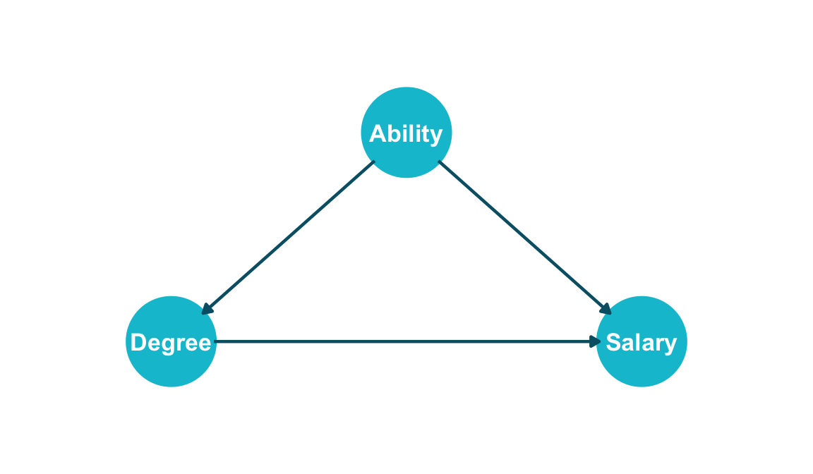
A Directed Acyclic Graph (DAG) consists of:

• Nodes = random variables
• Directed edges (arrows) = direct causal effects
• Acyclic = no feedback loops (no variable causes itself)

A DAG represents your qualitative causal assumptions about the data-generating process (Pearl 2009; Elwert 2013). It is not learned from data (that is Session 03) — it comes from domain knowledge.

library(ggdag)
library(ggplot2)

coord_dag <- list(
  x = c(Degree = 0, Ability = 0.5, Salary = 1),
  y = c(Degree = 0, Ability = 0.5, Salary = 0)
)

dag <- dagify(Degree ~ Ability,
              Salary ~ Degree,
              Salary ~ Ability,
              coords = coord_dag)

dag |>
  ggplot(aes(x = x, y = y, xend = xend, yend = yend)) +
  geom_dag_point(colour = "#00C1D4", size = 22) +
  geom_dag_edges(edge_colour = "#005e73", edge_width = 0.8) +
  geom_dag_text(colour = "white", size = 4.5, fontface = "bold") +
  expand_limits(x = c(-0.2, 1.2), y = c(-0.2, 0.7)) +
  coord_cartesian(clip = "off") +
  theme_dag(legend.position = "none")

Introduce the three defining properties of a DAG. Nodes are variables, directed edges represent direct causal effects, and acyclicity means no variable can be its own ancestor. The example shows a classic personnel economics DAG: ability causes both the university degree a person obtains and their salary, while the degree also has a direct effect on salary. Ability is a confounder. Emphasize that drawing a DAG is an act of encoding assumptions, not discovering facts. Two analysts with different domain knowledge may draw different DAGs for the same problem. The DAG is a tool for reasoning about the consequences of your assumptions. Mention dagitty.net as a practical tool students can use immediately.

A DAG is a non-parametric claim about independence structure

A DAG encodes three interconnected assumptions about the joint distribution:

Local Markov Assumption

Given its parents, each node is independent of all its non-descendants: \(X_i \perp\!\!\!\perp \text{NonDesc}(X_i) \mid \text{Pa}(X_i)\)

Minimality Assumption (Faithfulness)

Every edge in the DAG corresponds to a real dependence. Adjacent nodes are not independent given any subset of other nodes. No edges are superfluous — if you can remove an edge without violating any conditional independence, the DAG is wrong.

Causal Edge Assumption

Directed edges represent direct causal effects, not mere statistical associations. An outcome \(Y\) “listens to” its parents: \(Y\) changes in response to changes in its causes (Pearl 2009). This is what turns a Bayesian network into a causal model.

The first two assumptions imply the Bayesian network factorization (next slide); the third makes it causal.

This is a dense but essential slide. The Local Markov Assumption says that a node’s parents screen it off from the rest of the graph. This is what makes DAGs useful for reading off conditional independences. The Minimality Assumption is the converse: if the DAG includes an edge, the corresponding dependence must actually exist in the data. Without minimality, we could add edges everywhere and trivially satisfy the Markov condition. The Causal Edge Assumption is what separates a causal DAG from a generic Bayesian network. In a Bayesian network, edges encode factorization; in a causal DAG, they encode direct causal effects. This is what allows us to reason about interventions. The factorization formula decomposes the joint distribution into a product of conditionals, each node given its parents. This is both computationally and conceptually powerful.

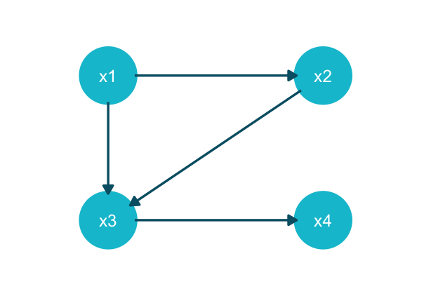
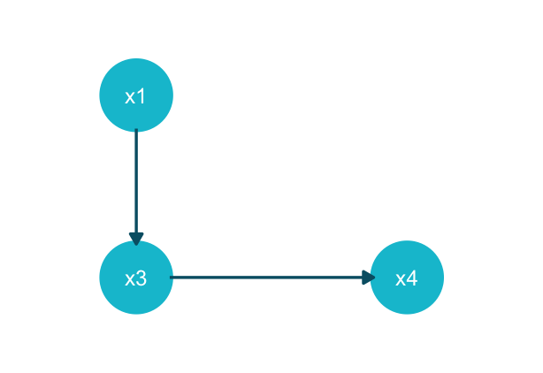
Bayesian network factorization turns an exponential joint into local pieces

By the chain rule of probability, any joint distribution factorizes as \[P(x_1, x_2, \ldots, x_n) = P(x_1) \prod_{i=2}^{n} P(x_i \mid x_{i-1}, \ldots, x_1)\]

For \(n = 4\) binary variables, the last term \(P(x_4 \mid x_3, x_2, x_1)\) alone requires \(2^{4-1} = 8\) parameters. A DAG exploits local dependencies via the Local Markov Assumption — we only condition on each node’s parents:

\(P_{\text{joint}} = P(x_1)\,P(x_2 \mid x_1)\,P(x_3 \mid x_2, x_1)\,P(x_4 \mid x_3)\)

\(P_{\text{joint}} = P(x_1)\,P(x_2)\,P(x_3 \mid x_1)\,P(x_4 \mid x_3)\)

This slide makes the “simplification” of the factorization concrete. Start with the chain rule of probability: any joint distribution factorizes as a product of conditionals over the full history. For four binary variables, the last term alone needs 8 parameters. The Local Markov Assumption lets us replace “conditioned on all previous variables” with “conditioned on parents only.” The two side-by-side DAGs show this: the left is dense (x3 has two parents) and yields a factorization with more terms; the right is sparse (x2 has no parents, x3 has only x1) and factorizes into simpler conditionals. The picture students should carry forward: every edge you add is a parameter commitment; every edge you can justifiably omit is a savings. The DAG’s structure encodes the simplification directly.

DAGs generate testable predictions

A DAG doesn’t just encode assumptions — it makes those assumptions falsifiable. Each DAG implies a full list of conditional independencies: every triple \((X, Y, Z)\) for which the graph claims \(X \perp\!\!\!\perp Y \mid Z\).

If data violates any of these, the DAG is likely misspecified.

The next two sections give us the machinery — building blocks (chain / fork / collider) and d-separation — to read these predictions off any DAG. The R/Python output on the right is a teaser of what we will then be able to compute and test.

Session 03 preview: Causal discovery algorithms reverse this logic — they test conditional independencies in data to learn the DAG.

Implied conditional independencies:

• R
• Python

library(dagitty)

dag <- dagitty("dag{
  Z1 -> D
  Z2 -> D
  Z2 -> Z3
  D -> M -> Y
  Z3 -> Y
  D -> Z4
  Y -> Z4
}")

print(impliedConditionalIndependencies(dag))

D _||_ Y | M, Z3
D _||_ Y | M, Z2
D _||_ Z3 | Z2
M _||_ Z1 | D
M _||_ Z2 | D
M _||_ Z3 | Z2
M _||_ Z3 | D
M _||_ Z4 | D, Y
Y _||_ Z1 | D, Z2
Y _||_ Z1 | D, Z3
Y _||_ Z1 | M, Z2
Y _||_ Z1 | M, Z3
Y _||_ Z2 | D, Z3
Y _||_ Z2 | M, Z3
Z1 _||_ Z2
Z1 _||_ Z3
Z1 _||_ Z4 | D, Y
Z1 _||_ Z4 | D, Z3
Z1 _||_ Z4 | D, Z2
Z2 _||_ Z4 | D, Y
Z2 _||_ Z4 | D, Z3
Z3 _||_ Z4 | D, Y
Z3 _||_ Z4 | M, Y, Z2

from pgmpy.base import DAG

dag = DAG([
    ("Z1", "D"), ("Z2", "D"), ("Z2", "Z3"),
    ("D", "M"), ("M", "Y"), ("Z3", "Y"),
    ("D", "Z4"), ("Y", "Z4")
])

print(dag.get_independencies())

(M ⟂ Z3 | D)
(Z1 ⟂ Z2)
(Y ⟂ Z1 | M, Z3)
(Z2 ⟂ Z4 | D, Y)
(Z3 ⟂ Z4 | D, Y)
(Z1 ⟂ Z4 | D, Y)
(M ⟂ Z2 | D)
(D ⟂ Y | M, Z3)
(Z1 ⟂ Z3)
(M ⟂ Z4 | D, Y)
(Y ⟂ Z2 | M, Z3)
(M ⟂ Z1 | D)
(D ⟂ Z3 | Z2)

Closes the “what is a DAG” arc with falsifiability as the third property (after “encodes assumptions” and “implies a factorization”). The live code is shown as a teaser — students cannot yet understand how impliedConditionalIndependencies() produces this list, but they can see that a DAG yields a concrete, finite set of testable claims. That motivates the next two sections (Building Blocks → d-Separation), where the machinery for reading these predictions off any DAG is introduced. The Session 03 hook closes the loop: causal discovery algorithms run this logic in reverse to learn DAGs from data.

Building Blocks of Association

Three structures govern every path in a DAG

Transition into the core graphical building blocks. Every path in a DAG is composed of exactly three elementary structures: chains, forks, and colliders. Understanding how each transmits or blocks statistical association is the key to reading off conditional independences from any DAG, no matter how complex.

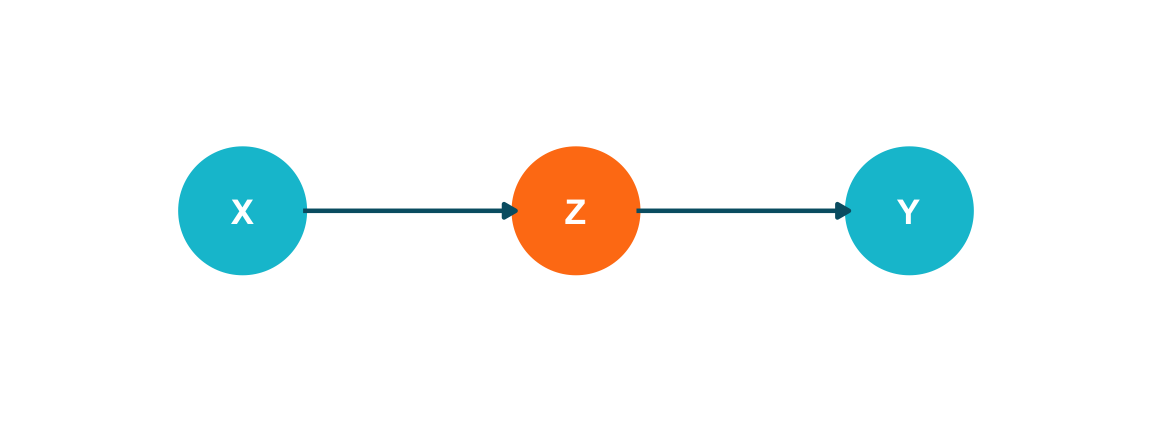
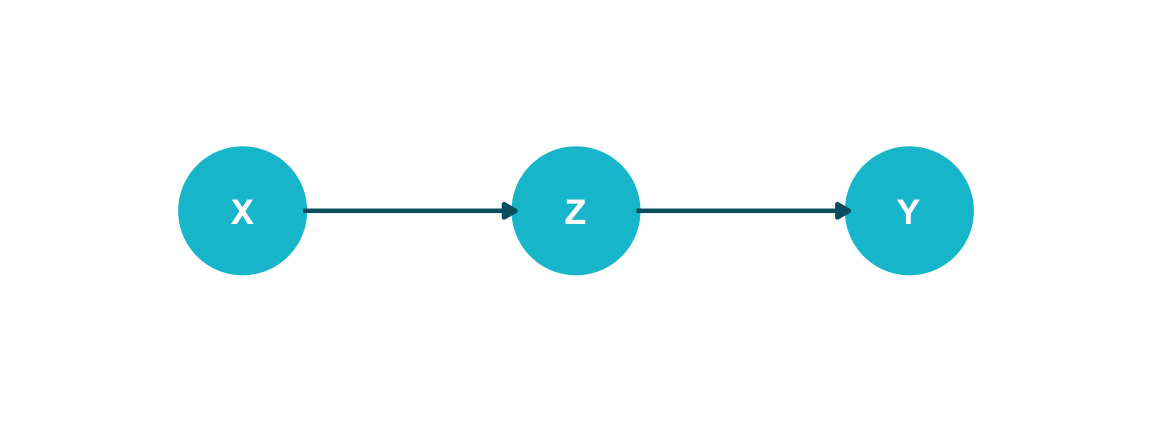
A chain transmits association from cause to effect

Chain: \(X \rightarrow Z \rightarrow Y\)

Association flows from \(X\) to \(Y\) through \(Z\). Here \(Z\) is a mediator.

Business example: R&D spending (\(X\)) \(\rightarrow\) product quality (\(Z\)) \(\rightarrow\) market share (\(Y\)).

Rule: A chain is open unconditionally. Conditioning on \(Z\) blocks the path: \[X \perp\!\!\!\perp Y \mid Z \;\Rightarrow\; P(X, Y \mid Z) = P(X \mid Z)\,P(Y \mid Z)\]

Unconditioned — path open

Conditioned on Z — path blocked

The chain is the simplest structure. X causes Z, and Z causes Y. Because Z transmits the effect of X to Y, X and Y are associated (the path is open, top DAG). Conditioning on Z (bottom DAG, Z shown in orange) blocks the path: with Z held constant, there is no remaining mechanism by which X can influence Y. The business example: if we hold product quality fixed, R&D spending tells us nothing additional about market share (assuming this is the only path).

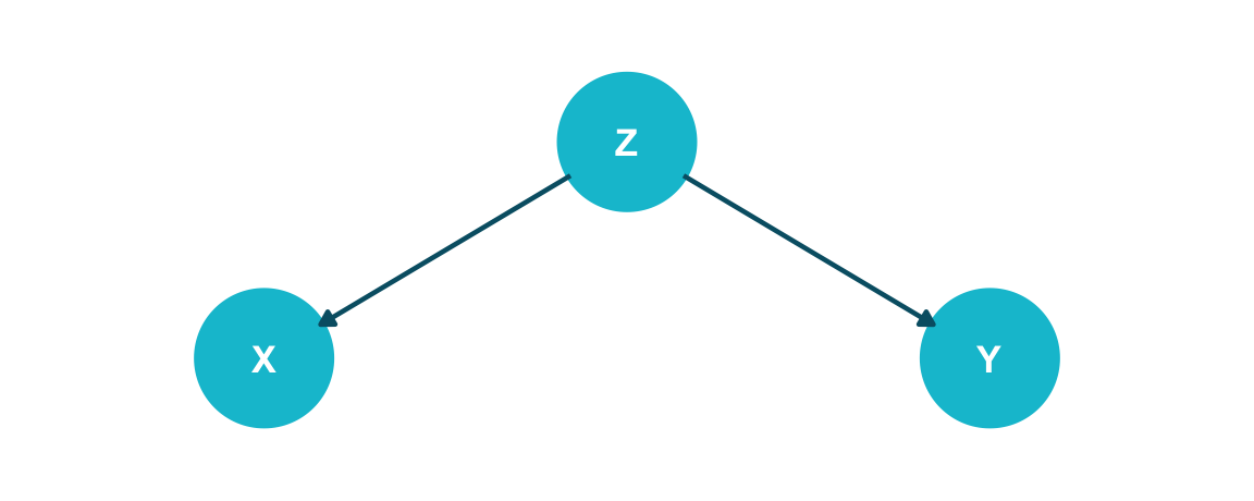
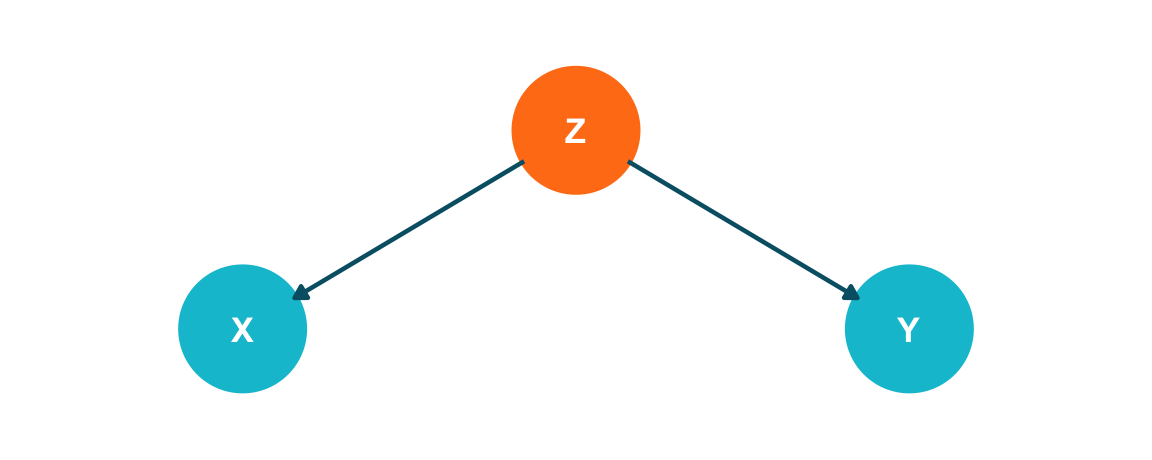
A fork creates spurious association through a common cause

Fork: \(X \leftarrow Z \rightarrow Y\)

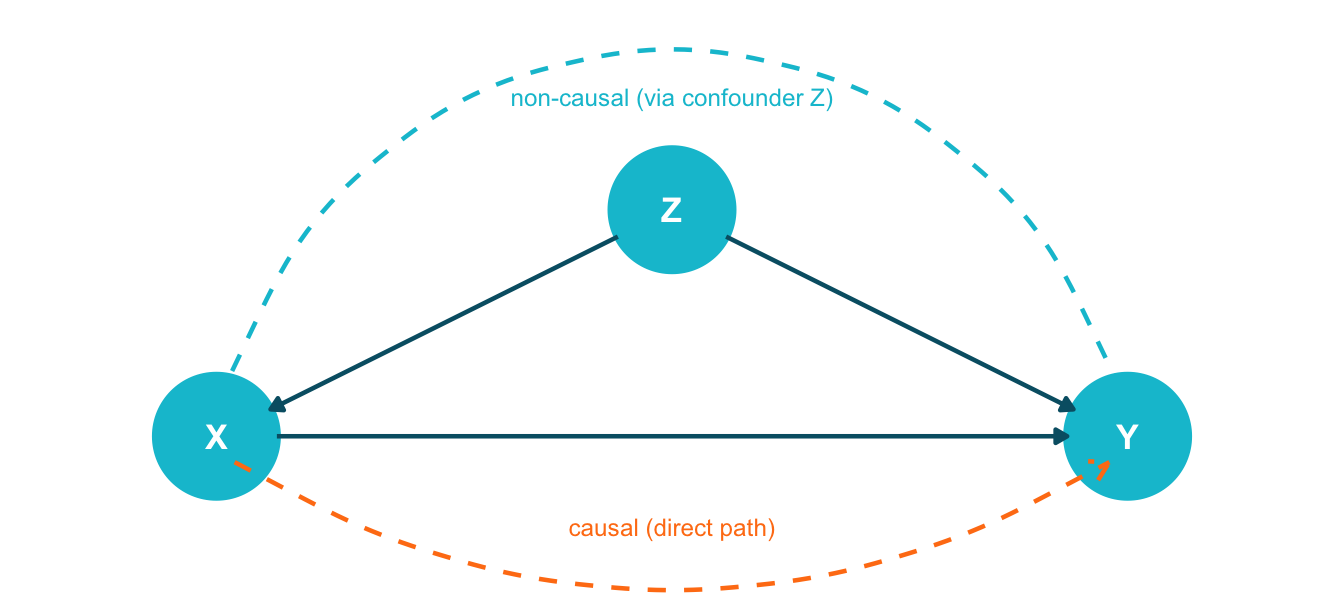
\(Z\) is a common cause — a confounder — that induces non-causal association between \(X\) & \(Y\).

Business example: Economic conditions (\(Z\)) affect both advertising spend (\(X\)) and revenue (\(Y\)). The observed correlation between ads and revenue is partly spurious.

Rule: A fork is open unconditionally. Conditioning on \(Z\) blocks the path: \[X \perp\!\!\!\perp Y \mid Z \;\Rightarrow\; P(X, Y \mid Z) = P(X \mid Z)\,P(Y \mid Z)\]

Unconditioned — path open

Conditioned on Z — path blocked

The fork is the classic confounding structure. Z causes both X and Y, creating a statistical association between X and Y even though neither causes the other. This is exactly the confounding we discussed in Session 01. The advertising-revenue example: during economic booms, companies spend more on ads AND revenue goes up. Observing a correlation between ads and revenue does not mean ads caused the revenue — economic conditions caused both. Conditioning on Z (bottom DAG, Z shown in orange) blocks the spurious path, isolating the genuine causal relationship (if any) between X and Y. The rule is the same as for chains: conditioning on the middle node blocks the path.

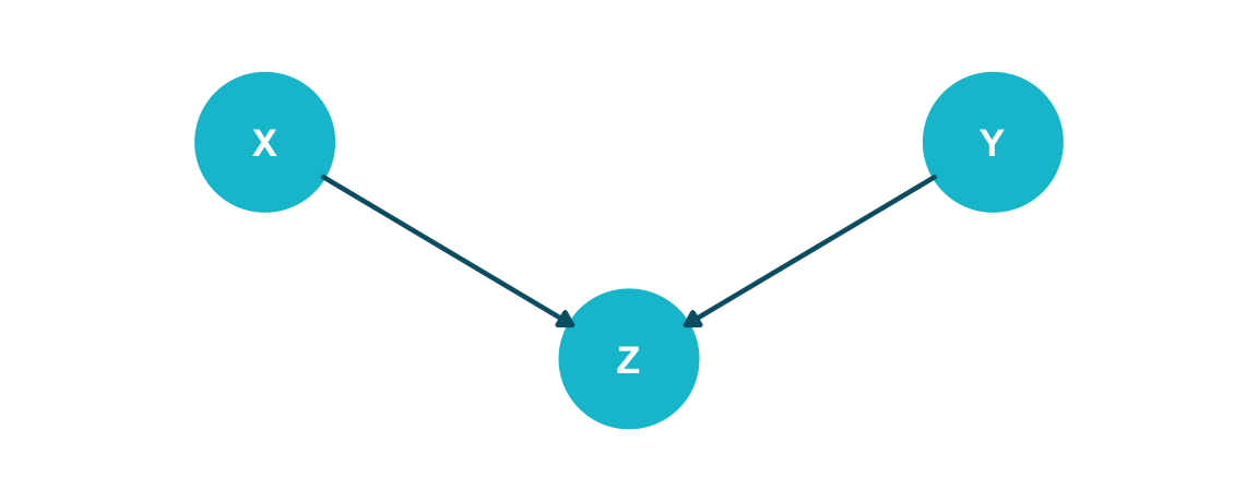
A collider blocks association — until you condition on it

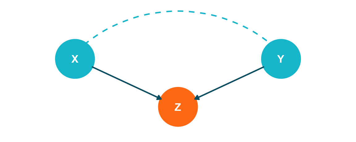
Collider (v-structure): \(X \rightarrow Z \leftarrow Y\)

Both arrows point into \(Z\), making it a collider. Unlike chains and forks, a collider blocks the path by default.

Berkson’s paradox: Looks (\(X\)) & talent (\(Y\)) are independent in the population, but both raise the chance of success (\(Z\): casting, funding, relationships). Among the successful, they appear negatively correlated.

Rule: A collider is blocked unconditionally, so \(X \perp\!\!\!\perp Y \Rightarrow P(X, Y) = P(X)\,P(Y)\). Conditioning on \(Z\) opens the path: \(X \not\perp\!\!\!\perp Y \mid Z\).

Unconditioned — path blocked

Conditioned on Z — path opens

The collider is the structure that surprises people. Two arrows pointing into the same node create a collision. Unlike chains and forks, a collider blocks the path by default (top DAG). X and Y are independent unconditionally. Conditioning on the collider Z (bottom DAG, Z in orange, dashed teal curve showing the newly opened path) creates a spurious association. Berkson’s paradox with looks × talent: both independent in the population, but among the successful they appear negatively correlated — if someone succeeded despite being plain-looking, they must be exceptionally talented. The rule is the opposite of chains and forks: leave it alone.

The collider trap: why “controlling for everything” can backfire

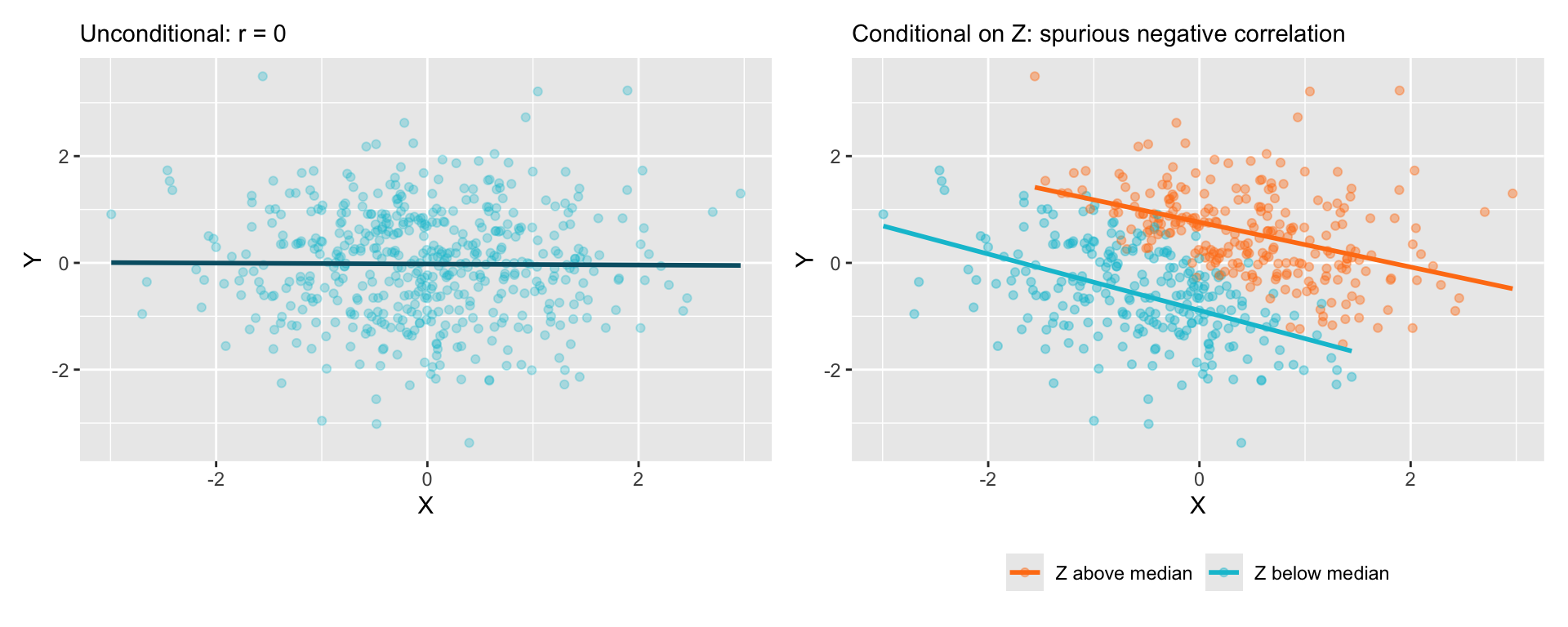
\(X\) and \(Y\) are independent causes of \(Z\). Unconditionally, \(X\) and \(Y\) are uncorrelated. But conditioning on \(Z\) (e.g., restricting to a subpopulation) creates a spurious correlation.

library(ggplot2)

set.seed(42)
n <- 500
x <- rnorm(n)
y <- rnorm(n)
z <- x + y + rnorm(n, sd = 0.3)

df <- data.frame(X = x, Y = y, Z = z,
                 group = ifelse(z > median(z), "Z above median", "Z below median"))

p1 <- ggplot(df, aes(x = X, y = Y)) +
  geom_point(alpha = 0.3, colour = "#00C1D4", size = 1.5) +
  geom_smooth(method = "lm", se = FALSE, colour = "#005e73", linewidth = 1) +
  labs(title = "Unconditional: r = 0",
       x = "X", y = "Y") +
  theme(plot.title = element_text(size = 11))

p2 <- ggplot(df, aes(x = X, y = Y, colour = group)) +
  geom_point(alpha = 0.4, size = 1.5) +
  geom_smooth(method = "lm", se = FALSE, linewidth = 1) +
  scale_colour_manual(values = c("Z above median" = "#FF7E15",
                                 "Z below median" = "#00C1D4")) +
  labs(title = "Conditional on Z: spurious negative correlation",
       x = "X", y = "Y", colour = NULL) +
  theme(plot.title = element_text(size = 11),
        legend.position = "bottom")

library(patchwork)
p1 + p2

The mantra “control for everything available” is not just wrong — it is dangerous. Including a collider as a control variable introduces bias where none existed.

This simulation makes the collider trap visceral. X and Y are generated independently, so the unconditional correlation is essentially zero. But Z is caused by both X and Y. When we split the data by Z (above/below median), a strong negative correlation appears within each subgroup. If X was high and Z is at a fixed level, then Y must have been low, and vice versa. This is Berkson’s paradox in action. The left panel shows the truth: X and Y are independent. The right panel shows the artifact: within strata of Z, they appear negatively correlated. The message for practitioners: never add control variables reflexively. Each variable must be evaluated for its causal role. Colliders and their descendants should be left out. This is why we need DAGs.

Conditioning on a descendant of a collider also opens the path

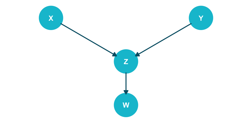
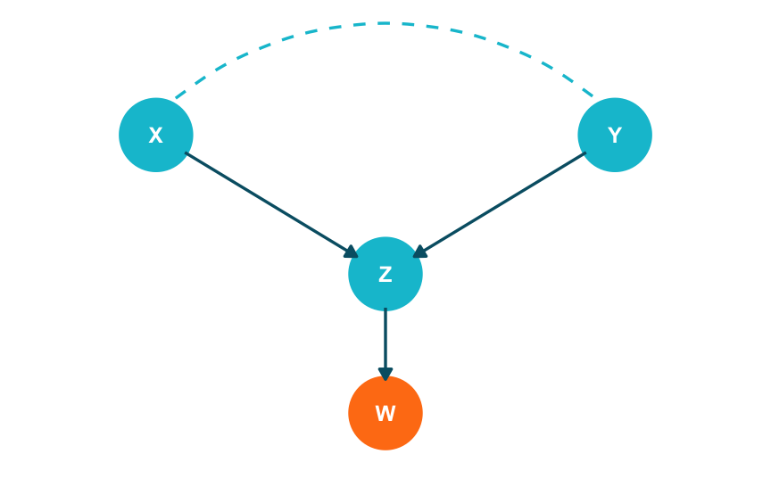
Conditioning on a descendant of a collider partially opens the collider path — information about the descendant leaks information about the collider itself.

Extended example: Programming skill (\(X\)) \(\rightarrow\) Hired (\(Z\)) \(\leftarrow\) Social skill (\(Y\)), and Hired (\(Z\)) \(\rightarrow\) Team assignment (\(W\)).

Rule: The path \(X \to Z \leftarrow Y\) is blocked when we do not condition on \(Z\) or any of its descendants. Conditioning on \(W\) (a descendant of \(Z\)) opens the path: \(X \not\perp\!\!\!\perp Y \mid W\).

Unconditioned — collider path blocked

Conditioned on descendant W — path opens

This slide extends the collider rule. Conditioning on a descendant of a collider also opens the collider path, though the induced association is typically weaker. In the example, team assignment depends on whether someone was hired, which depends on both programming and social skills. If we study the relationship between programming and social skill among people in team A, we are implicitly selecting on a descendant of the hiring decision, which opens the collider path. This is subtle but practically important: many post-treatment variables are descendants of colliders, and including them as controls can introduce bias.

The three rules summarized

Structure	Pattern	Role of Z	Unconditional	Conditioned on Z	Action
Chain	\(X \rightarrow Z \rightarrow Y\)	Mediator	Open	Blocked	Do NOT adjust (blocks causal path)
Fork	\(X \leftarrow Z \rightarrow Y\)	Confounder	Open	Blocked	DO adjust (removes spurious path)
Collider	\(X \rightarrow Z \leftarrow Y\)	Collider	Blocked	Opened	Do NOT adjust (opens spurious path)

Key takeaway: Chains and forks — condition to block. Colliders — condition to open. Every complex DAG reduces to combinations of these three structures.

This summary table is one students should memorize. Chains and forks behave identically: open by default, blocked by conditioning. Colliders are the opposite: blocked by default, opened by conditioning. This asymmetry is the source of most confusion in applied causal inference. The practical rule is simple: if you see two arrows pointing into the same node (collider), do not condition on it or its descendants. If you see a common cause (fork) or a mediator (chain), conditioning blocks the path. Every path in any DAG, no matter how complex, is a sequence of these three structures. Checking whether a path is open or blocked reduces to checking each triple along the path.

d-Separation

Real DAGs have dozens of paths. We need an algorithm, not intuition.

Transition slide. The three building blocks are sufficient for simple three-node DAGs, but real causal models have many variables and many paths between any two nodes. Checking each path manually is error-prone. d-separation provides a systematic algorithm for determining conditional independence from the graph structure alone. It generalizes the three building-block rules to arbitrary DAGs.

d-separation checks every path between two nodes simultaneously

Definition: d-separation

Two nodes \(X\) and \(Y\) are d-separated by a set \(Z\) (written \(X \perp\!\!\!\perp_{G} Y \mid Z\)) if and only if every path between \(X\) and \(Y\) is blocked by \(Z\).

A path is blocked by \(Z\) if it contains at least one of:

(a) A chain \(\ldots \rightarrow W \rightarrow \ldots\) or fork \(\ldots \leftarrow W \rightarrow \ldots\) where \(W \in Z\)

(b) A collider \(\ldots \rightarrow W \leftarrow \ldots\) where \(W \notin Z\) and no descendant of \(W\) is in \(Z\)

If \(X\) and \(Y\) are not d-separated by \(Z\), they are d-connected given \(Z\) — at least one open path remains.

Algorithm: For each path between \(X\) and \(Y\), check every triple. If all paths are blocked, the nodes are d-separated. If any path is open, they are d-connected.

State the formal definition carefully. d-separation requires that every single path between X and Y is blocked. A path is blocked if at least one node along it satisfies one of the two blocking conditions: either it is a non-collider that we condition on, or it is a collider that we do not condition on (and none of its descendants are conditioned on either). If even one path remains open, X and Y are d-connected given Z, meaning the graph predicts they will be statistically associated. The algorithm is mechanical: enumerate paths, check triples. In practice, software does this automatically, but understanding the logic is essential for building correct DAGs.

d-separation is a graphical test for conditional independence

Under the Local Markov and Faithfulness assumptions:

\[X \perp\!\!\!\perp_{G} Y \mid Z \quad \iff \quad X \perp\!\!\!\perp Y \mid Z\]

d-separation in the graph corresponds to conditional independence in the distribution.

Implications:

• Markov direction (\(\Rightarrow\)): If \(X\) and \(Y\) are d-separated by \(Z\) in the graph, then \(X \perp\!\!\!\perp Y \mid Z\) in every distribution compatible with the DAG.

• Faithfulness direction (\(\Leftarrow\)): If \(X \perp\!\!\!\perp Y \mid Z\) in the distribution, then \(X\) and \(Y\) are d-separated by \(Z\) in the graph. (No “accidental” cancellations.)

This correspondence is what makes DAGs useful for causal inference: graphical structure \(\leftrightarrow\) statistical testable predictions. Violations suggest the DAG is misspecified.

This slide establishes the bridge between graph theory and probability theory. The Markov direction is guaranteed by the Local Markov Assumption: d-separation implies conditional independence. The Faithfulness direction adds the converse: every conditional independence in the data corresponds to a d-separation in the graph. Faithfulness rules out pathological cases where two paths exactly cancel each other’s associations. This bidirectional correspondence is what makes DAGs testable: we can check the implied conditional independences against data. If a predicted independence fails empirically, the DAG may be wrong. This testability is a major advantage over purely verbal causal reasoning. Session 03 on causal discovery exploits this correspondence to learn DAGs from data.

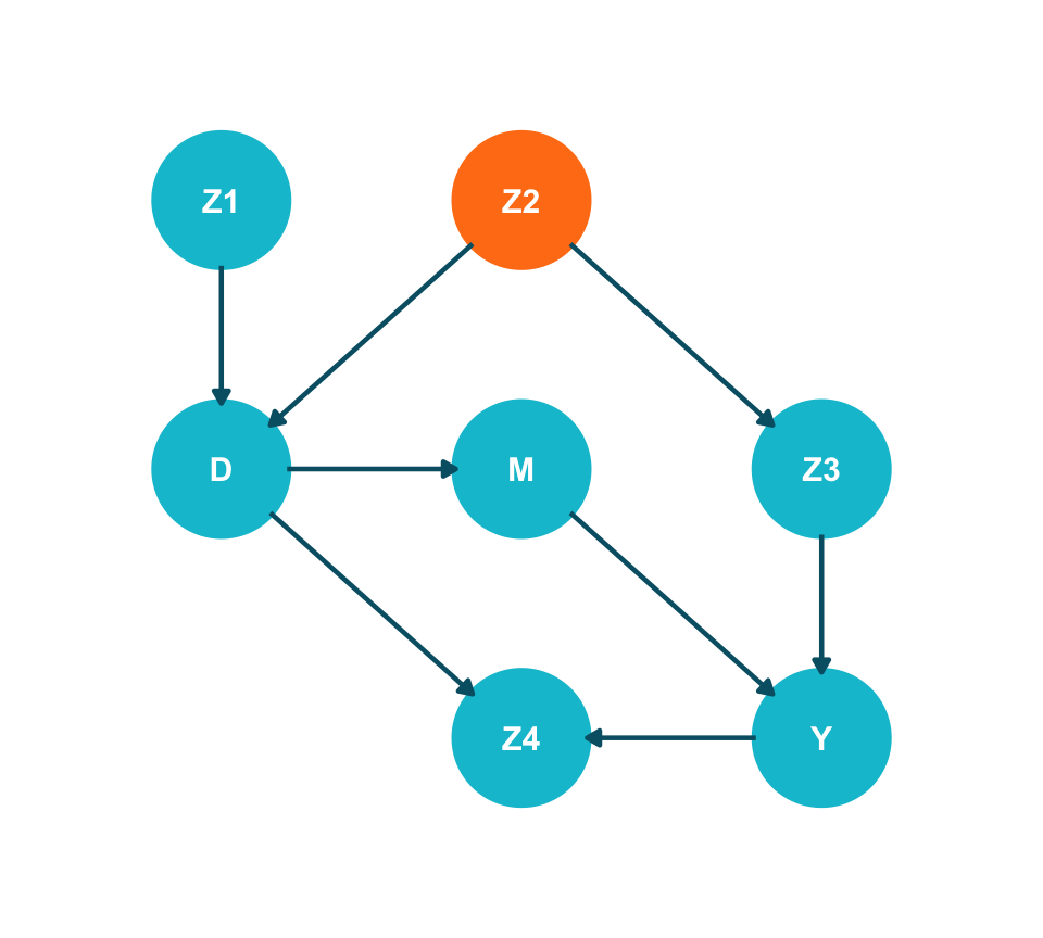
Worked example: Is \(D \perp\!\!\!\perp_{G} Y \mid \{Z2\}\)?

library(ggdag)
library(ggplot2)

coord_dag <- list(
  x = c(Z1 = 0, Z2 = 0.5, D = 0, Z3 = 1, M = 0.5, Y = 1, Z4 = 0.5),
  y = c(Z1 = 1, Z2 = 1, D = 0.5, Z3 = 0.5, M = 0.5, Y = 0, Z4 = 0)
)

dag <- dagify(
  D ~ Z1,
  D ~ Z2,
  Z3 ~ Z2,
  M ~ D,
  Y ~ M,
  Y ~ Z3,
  Z4 ~ D,
  Z4 ~ Y,
  coords = coord_dag
)

dag_data <- dag |> tidy_dagitty()
dag_data$data$colour <- ifelse(dag_data$data$name == "Z2",
                               "#FF7E15", "#00C1D4")

dag_data |>
  ggplot(aes(x = x, y = y, xend = xend, yend = yend)) +
  geom_dag_point(aes(colour = colour), size = 22) +
  scale_colour_identity() +
  geom_dag_edges(edge_colour = "#005e73", edge_width = 0.8) +
  geom_dag_text(colour = "white", size = 4, fontface = "bold") +
  expand_limits(x = c(-0.2, 1.2), y = c(-0.2, 1.2)) +
  coord_cartesian(clip = "off") +
  theme_dag(legend.position = "none")

Paths from \(D\) to \(Y\):

1. \(D \rightarrow M \rightarrow Y\) (chain — open, no conditioned node)
2. \(D \leftarrow Z2 \rightarrow Z3 \rightarrow Y\) (fork at Z2 — blocked by conditioning on Z2)
3. \(D \rightarrow Z4 \leftarrow Y\) (collider at Z4 — blocked, Z4 not conditioned on)

Path 1 is open \(\Rightarrow\) d-connected. \(D \not\perp\!\!\!\perp_{G} Y \mid \{Z2\}\).

First conditioning set. The DAG has 7 nodes and three paths between D and Y. Ask students to work through it before revealing. Path 1 through M is a chain with no conditioned node, so it is open. Path 2 has a fork at Z2, and since Z2 is in the conditioning set, this path is blocked. Path 3 has a collider at Z4, which is not conditioned on, so it is blocked by default. Since path 1 remains open, D and Y are d-connected given Z2. Conditioning on Z2 alone is not sufficient.

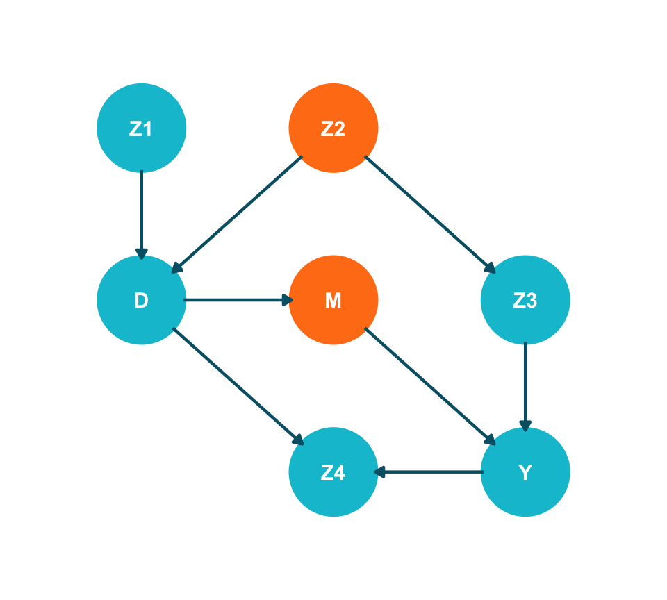
Worked example: Is \(D \perp\!\!\!\perp_{G} Y \mid \{Z2, M\}\)?

library(ggdag)
library(ggplot2)

coord_dag <- list(
  x = c(Z1 = 0, Z2 = 0.5, D = 0, Z3 = 1, M = 0.5, Y = 1, Z4 = 0.5),
  y = c(Z1 = 1, Z2 = 1, D = 0.5, Z3 = 0.5, M = 0.5, Y = 0, Z4 = 0)
)

dag <- dagify(
  D ~ Z1,
  D ~ Z2,
  Z3 ~ Z2,
  M ~ D,
  Y ~ M,
  Y ~ Z3,
  Z4 ~ D,
  Z4 ~ Y,
  coords = coord_dag
)

dag_data <- dag |> tidy_dagitty()
dag_data$data$colour <- ifelse(dag_data$data$name %in% c("Z2", "M"),
                               "#FF7E15", "#00C1D4")

dag_data |>
  ggplot(aes(x = x, y = y, xend = xend, yend = yend)) +
  geom_dag_point(aes(colour = colour), size = 22) +
  scale_colour_identity() +
  geom_dag_edges(edge_colour = "#005e73", edge_width = 0.8) +
  geom_dag_text(colour = "white", size = 4, fontface = "bold") +
  expand_limits(x = c(-0.2, 1.2), y = c(-0.2, 1.2)) +
  coord_cartesian(clip = "off") +
  theme_dag(legend.position = "none")

1. \(D \rightarrow M \rightarrow Y\) — blocked (M conditioned on)
2. \(D \leftarrow Z2 \rightarrow Z3 \rightarrow Y\) — blocked (Z2 conditioned on)
3. \(D \rightarrow Z4 \leftarrow Y\) — blocked (collider, Z4 not conditioned on)

All paths blocked \(\Rightarrow\) d-separated. \(D \perp\!\!\!\perp_{G} Y \mid \{Z2, M\}\).

Second conditioning set. Now we add M to the conditioning set. Path 1 through M is a chain and M is conditioned on, so it is blocked. Path 2 remains blocked by Z2. Path 3 is still a collider with Z4 not conditioned on, so it remains blocked. All three paths are now blocked, so D and Y are d-separated given Z2 and M. Note that conditioning on M blocks the causal path from D to Y — this would be problematic if we wanted to estimate the total effect, but it correctly achieves d-separation. Highlight the conditioned nodes in orange on the DAG.

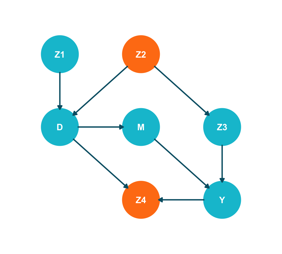
Worked example: Is \(D \perp\!\!\!\perp_{G} Y \mid \{Z2, Z4\}\)?

library(ggdag)
library(ggplot2)

coord_dag <- list(
  x = c(Z1 = 0, Z2 = 0.5, D = 0, Z3 = 1, M = 0.5, Y = 1, Z4 = 0.5),
  y = c(Z1 = 1, Z2 = 1, D = 0.5, Z3 = 0.5, M = 0.5, Y = 0, Z4 = 0)
)

dag <- dagify(
  D ~ Z1,
  D ~ Z2,
  Z3 ~ Z2,
  M ~ D,
  Y ~ M,
  Y ~ Z3,
  Z4 ~ D,
  Z4 ~ Y,
  coords = coord_dag
)

dag_data <- dag |> tidy_dagitty()
dag_data$data$colour <- ifelse(dag_data$data$name %in% c("Z2", "Z4"),
                               "#FF7E15", "#00C1D4")

dag_data |>
  ggplot(aes(x = x, y = y, xend = xend, yend = yend)) +
  geom_dag_point(aes(colour = colour), size = 22) +
  scale_colour_identity() +
  geom_dag_edges(edge_colour = "#005e73", edge_width = 0.8) +
  geom_dag_text(colour = "white", size = 4, fontface = "bold") +
  expand_limits(x = c(-0.2, 1.2), y = c(-0.2, 1.2)) +
  coord_cartesian(clip = "off") +
  theme_dag(legend.position = "none")

1. \(D \rightarrow M \rightarrow Y\) — open (M not conditioned on)
2. \(D \leftarrow Z2 \rightarrow Z3 \rightarrow Y\) — blocked (Z2 conditioned on)
3. \(D \rightarrow Z4 \leftarrow Y\) — opened (collider Z4 conditioned on!)

d-connected via two open paths. Conditioning on Z4 made things worse.

Third conditioning set — the trap. Replacing M with Z4 in the conditioning set has two consequences. Path 1 through M is no longer blocked because M is not conditioned on. But more importantly, path 3, which was previously blocked because Z4 is a collider, is now opened because we condition on Z4. So we go from one open path to two open paths. Adding Z4 to the conditioning set increased the number of associations between D and Y rather than decreasing it. This is the collider trap in a complex DAG — exactly the phenomenon we demonstrated with the simulation earlier. The lesson: conditioning on a collider or its descendant opens a previously blocked path.

Software verifies d-separation instantly

R: dagitty + ggdag   |   Python: pgmpy   |   Browser: dagitty.net

• R
• Python

library(dagitty)

dag <- dagitty("dag{
  Z1 -> D
  Z2 -> D
  Z2 -> Z3
  D -> M -> Y
  Z3 -> Y
  D -> Z4
  Y -> Z4
}")

cat("D _||_ Y | {Z2}?       ", dseparated(dag, "D", "Y", "Z2"), "\n")

D _||_ Y | {Z2}?        FALSE 

cat("D _||_ Y | {Z2, M}?    ", dseparated(dag, "D", "Y", c("Z2", "M")), "\n")

D _||_ Y | {Z2, M}?     TRUE 

cat("D _||_ Y | {Z2, Z4}?   ", dseparated(dag, "D", "Y", c("Z2", "Z4")), "\n")

D _||_ Y | {Z2, Z4}?    FALSE 

from pgmpy.base import DAG

dag = DAG([
    ("Z1", "D"), ("Z2", "D"), ("Z2", "Z3"),
    ("D", "M"), ("M", "Y"), ("Z3", "Y"),
    ("D", "Z4"), ("Y", "Z4")
])

print("D ⊥ Y | {Z2}?      ",
      not dag.is_dconnected("D", "Y", observed=["Z2"]))

D ⊥ Y | {Z2}?       False

print("D ⊥ Y | {Z2, M}?   ",
      not dag.is_dconnected("D", "Y", observed=["Z2", "M"]))

D ⊥ Y | {Z2, M}?    True

print("D ⊥ Y | {Z2, Z4}?  ",
      not dag.is_dconnected("D", "Y", observed=["Z2", "Z4"]))

D ⊥ Y | {Z2, Z4}?   False

After the manual worked examples, show students that software does the heavy lifting. The dseparated function in R (or is_dconnected in pgmpy, negated) confirms our manual path-by-path analysis. Encourage students to always verify their reasoning computationally. Note the pgmpy API quirk: is_dconnected returns True when connected, so we negate it to match dagitty’s dseparated convention. Both packages define the DAG the same way — as a list of directed edges.

Flow of association and causation — the big picture

• Total association between two variables flows along all unblocked paths in a DAG.
  • Association along directed unblocked paths is causal — asymmetric, a subset of total association.
  • The rest is non-causal: confounding or selection bias — symmetric, not the target of inference.
• d-separation lets us ask: “Ignoring the causal paths, are \(X\) and \(Y\) d-separated otherwise?” If yes, observed association equals causal effect.

Capstone slide for the d-Separation section. The diagram shows a single DAG (fork + direct path) with two coloured association curves: the orange “causal” flow goes directly from X to Y, while the teal “non-causal” flow loops up through the confounder Z. Students should carry forward this mental picture: identification is the art of closing the teal arrow while keeping the orange one open. Every backdoor/frontdoor/do-calculus rule we will see is a recipe for this surgical separation. This positions the Backdoor Criterion as the first concrete recipe.

The do-Operator

Before identifying causal effects, we need to be precise about what an intervention is.

Transition into the do-operator section. d-Separation gave us a way to read conditional independencies off any DAG; now we need a tool that goes one step further — that lets us reason about what would happen if we acted on a variable rather than just observed it. The do-operator is exactly that tool. The next three slides establish (i) that conditioning and intervention are different distributions, (ii) what intervention means graphically (graph surgery), and (iii) why the two distributions differ mechanically (the factorization swap). Backdoor adjustment, frontdoor adjustment, and the do-calculus rules all rest on this foundation.

Conditioning vs. intervention: two different distributions

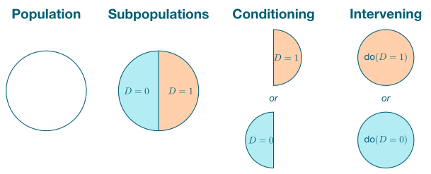
• Conditioning filters the data: keep only units with \(D = d\) (a half-population). Their covariate distribution \(P(X \mid D = d)\) is generally not the population’s — it is contaminated by whatever pushed those units toward \(D = d\).
• Intervention sets \(D = d\) for everyone (the full population): the rest of the system (in particular \(P(X)\)) is left intact. Graphically, the arrow \(X \rightarrow D\) is severed.
• The two distributions coincide only in special cases: no confounding (no \(X \rightarrow D\) to begin with), an RCT (randomization breaks \(X \rightarrow D\) by design), or a satisfied identification criterion (we reconstruct the interventional distribution from observation + adjustment).

Adapted from Neal, B. (2020). Introduction to Causal Inference from a Machine Learning Perspective.

This TikZ rendering of Neal’s figure makes the conceptual contrast explicit. Left side: conditioning filters to a sub-population, dashed selection box highlights the restriction. Right side: intervention sets the value for everyone, the orange box and orange-coloured T node mark the intervention target, the dotted-grey X→T arrow with an orange × shows the graph surgery step. The interpretation bullets, revealed as a fragment, walk students through the two key takeaways: (i) conditioning corrupts the covariate distribution, (ii) intervention preserves it, and (iii) the two coincide only when there’s no confounding or when randomization or a graphical criterion lets us bridge them. This sets up the next two slides — graph surgery as the formal definition, and the factorization swap as the mechanical consequence.

Graph surgery shows what intervention really means

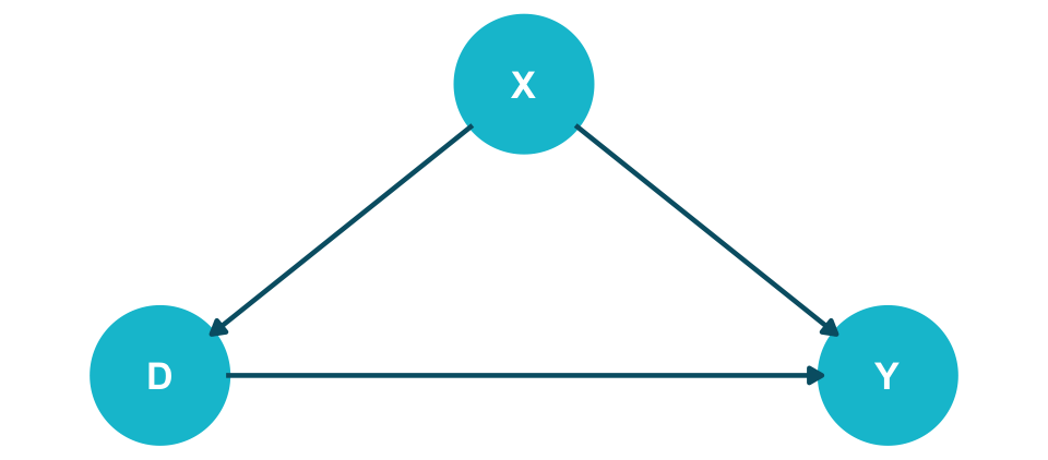
Observational graph \(G\):

When we simply observe \(D\), all arrows remain. \(D\) is determined by its causes (including confounders).

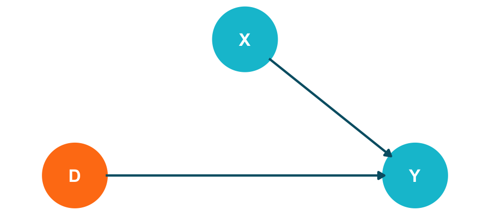
Mutilated graph \(G_{\overline{D}}\):

When we intervene on \(D\) (set \(D = d\)), we delete all arrows into \(D\). The intervention replaces whatever normally determines \(D\).

The do-operator is concrete: \(P(Y \mid do(D = d))\) is simply \(P(Y \mid D = d)\) in the mutilated graph \(G_{\overline{D}}\). Graph surgery severs the confounding, making \(D\) independent of \(X\). This is exactly what an RCT does in practice.

Many (if not most) real questions involve intervention, not prediction: \(P(\text{Performance} \mid do(\text{Training}))\), \(\;P(\text{Sales} \mid do(\text{Incentive}))\), \(\;P(\text{CTR} \mid do(\text{Ad}))\), \(\;P(\text{Churn} \mid do(\text{Call center}))\).

Graph surgery is the graphical counterpart of an intervention. In the observational graph, D is caused by X (the confounder), so observing D tells us something about X, which biases our estimate of D’s effect on Y. When we intervene on D, we set it to a specific value regardless of X. Graphically, this means deleting all arrows into D. In the mutilated graph, D has no parents, so it is independent of X. The do-operator simply computes regular conditional probabilities in this modified graph. The four business-example queries make the L1/L2 distinction tangible: every one of these is a decision, not a description. Pearl’s do-calculus generalizes this surgery to derive identification results for arbitrary DAGs.

Why conditioning ≠ intervention: factorizations differ

Observational (graph \(G\), all arrows intact):

\[P(X, D, Y) = P(X)\,\underbrace{P(D \mid X)}_{\text{cause of } D}\,P(Y \mid D, X)\]

Step 1 — Bayes for the weight on \(x\): \[\textcolor{#00C1D4}{P(X \mid D = d)} = \frac{P(X)\,P(D = d \mid X)}{P(D = d)}\]

Step 2 — chain rule for \((X, Y)\) given \(D = d\): \[P(X, Y \mid D = d) = P(Y \mid D = d, X)\,\textcolor{#00C1D4}{P(X \mid D = d)}\]

Step 3 — sum over \(x\) (law of total probability): \[P(Y \mid D = d) = \sum_x P(Y \mid D = d, X = x)\,\underbrace{\textcolor{#00C1D4}{P(X \mid D = d)}}_{\text{post-treatment weight}}\]

Interventional (graph \(G_{\overline{D}}\), \(do(D = d)\) deletes \(P(D \mid X)\)):

\[P(X, D, Y) = P(X)\,\cancel{P(D \mid X)}\,P(Y \mid D, X)\]

Step 1 — under intervention, \(X\) is unaffected: \[P(X \mid do(D = d)) = \textcolor{#FF7E15}{P(X)}\]

Step 2 — truncated joint of \((X, Y)\) at \(D = d\): \[P(X, Y \mid do(D = d)) = P(Y \mid D = d, X)\,\textcolor{#FF7E15}{P(X)}\]

Step 3 — sum over \(x\): \[P(Y \mid do(D = d)) = \sum_x P(Y \mid D = d, X = x)\,\underbrace{\textcolor{#FF7E15}{P(X)}}_{\text{natural weight}}\]

Same kernel \(P(Y \mid D = d, X)\) — only the weight on \(x\) differs: \(\textcolor{#00C1D4}{P(X \mid D = d)}\) vs. \(\textcolor{#FF7E15}{P(X)}\), equal iff \(X \perp\!\!\!\perp D\).

Now anchored to the same D, X, Y DAG as the previous slide. The derivation walks students through one mechanical step on each side. Observational: factorize the joint, marginalize X from \(P(Y \mid D = d)\) — out comes the weight \(P(X \mid D = d)\). Interventional: delete \(P(D \mid X)\) from the factorization (graph surgery), then marginalize X — out comes the weight \(P(X)\). Side-by-side, the two formulas are identical EXCEPT for which distribution of X is used to average. That single term — the conditional vs. marginal distribution of X — is the entire mathematical content of “correlation ≠ causation.” When there is no confounding (no \(X \rightarrow D\) to begin with) the two coincide; when randomization severs \(X \rightarrow D\) they coincide too; otherwise the two distributions are genuinely different. The next section turns this insight into a practical recipe — the backdoor criterion — which says: pick the set \(X\) of confounders carefully so that within strata, the conditional and marginal weights agree.

References

Elwert, Felix. 2013. “Graphical Causal Models.” In Handbook of Causal Analysis for Social Research, edited by Stephen L. Morgan, 245–73. Springer. https://doi.org/10.1007/978-94-007-6094-3_13.

Pearl, Judea. 2009. Causality: Models, Reasoning, and Inference. 2nd ed. Cambridge University Press. https://doi.org/10.1017/CBO9780511803161.

Thank you for your attention!
	www.startupengineer.io/team/ihl/ christoph-ihl christophihl