6 Session: Experiments & Linear Regression
6.1 Lecture Slides
6.2 Overview
Randomized controlled trials are the closest thing to a gold standard in causal inference: by construction, the treatment \(D\) becomes independent of every covariate, observed or unobserved, so the associational difference in means equals the causal ATE. This session formalises the claim through three complementary lenses — the do-calculus inherited from Session 03, the potential-outcomes bias decomposition, and exchangeability — then bridges to the linear regression that operationalises all three. The OLS coefficient on \(D\) in \(Y \sim D\) is exactly the difference of group means, so OLS is the natural estimator under randomization. We then equip you with the inferential machinery (heteroskedasticity-robust standard errors, t-tests, confidence intervals, the bootstrap, plus the Fisher-style randomization test as an exact alternative) to quantify uncertainty around \(\hat\tau\). Finally, OLS extends naturally to multivalued and continuous treatments and gives you a principled way to use pre-treatment covariates for variance reduction — the only legitimate role of covariates under randomization, since de-confounding is Session 06’s job.
The PBL works through five exercises: Christmas/socks (causal vs. associational ATE and the bias decomposition), an in-app feature rollout (manual SE/CI/HT, then OLS, then bootstrap and randomization-inference verification), blocked random assignment (variance reduction by design), the Lin (2013) covariate-adjusted estimator with a post-treatment collider trap, and a multivalued + continuous-treatments closing.
6.3 Lecture Notes
6.3.1 Randomization and covariate balance
A randomized assignment protocol draws each unit’s treatment value from a known distribution that does not depend on any of the unit’s other characteristics. For a \(k\)-armed trial with equal allocation, \(P(D_i = d) = 1/k\). For a binary trial with allocation probability \(p\), \(P(D_i = 1) = p\) and \(P(D_i = 0) = 1 - p\). The defining feature is that the assignment mechanism is known, coin-flip-like, and external to the unit.
This single feature is what makes randomization the cleanest causal-inference design. Let \(\mathbf{X}\) be any vector of pre-treatment characteristics — observed or unobserved. Because \(D\) is drawn from a coin flip independent of \(\mathbf{X}\), the joint distribution factorises: \(P(D, \mathbf{X}) = P(D) \cdot P(\mathbf{X})\). Equivalently, the conditional distribution of covariates given treatment does not depend on which arm was assigned:
\[P(\mathbf{X} \mid D = d) \;\stackrel{d}{=}\; P(\mathbf{X} \mid D = d') \quad \text{for all } d, d'.\]
This is covariate balance, and it is the same statement as the independence claim \(\mathbf{X} \perp\!\!\!\perp D\). Critically, the implication holds even when \(\mathbf{X}\) contains variables we never observe: the random number generator does not consult them either. This is the central reason RCTs dominate observational designs, where matching, regression adjustment, and IPW can balance only the covariates we have measured.
6.3.1.1 Blocked random assignment
In small samples, the realised covariate balance can drift noticeably from its expectation. Blocked random assignment (also called stratified randomization or, in the tech-industry vocabulary, stratified A/B testing) restores balance exactly on a chosen pre-treatment variable, by randomising independently within each level of that variable. If \(S_k\) indexes the strata (e.g., quartiles of pre-period spend, or the levels of a categorical demographic), the protocol is:
- Partition the sample by \(S\).
- Within each stratum \(S_k\), randomly assign half (or a chosen fraction) to \(D = 1\), the rest to \(D = 0\).
The stratified ATE estimator weights the within-stratum mean differences by stratum size:
\[\hat\tau_{\text{blocked}} \;=\; \sum_k \pi_k \big(\bar Y^{(1)}_k - \bar Y^{(0)}_k\big), \qquad \pi_k = n_k / n.\]
When \(S\) is predictive of \(Y\), this reduces residual variance and hence the standard error of \(\hat\tau\) — variance reduction by design. The slide deck’s worked example uses prior-period spend in a marketing experiment: blocking on its quartile pins down half the treated units in each quartile, eliminating the sample-to-sample variability in the realised quartile shares that simple randomization carries.
Blocking pairs naturally with the analysis-time covariate adjustment: blocking on a variable plus regression-adjusting on it is partly redundant; blocking on one set of variables and regression-adjusting on a different set is complementary. Modern A/B-testing platforms (Optimizely, GrowthBook, Statsig) block on user attributes by default, then layer covariate adjustment (and CUPED-style pre-experiment adjustment, S05) on top. Exercise 3 walks through a hands-on simulation contrasting simple and blocked SEs at the same point estimate.
6.3.2 Three perspectives on association → causation
Why does the simple difference of group means recover a causal effect under randomization? The slides walk through three perspectives. We restate each here and emphasise where they live in the broader course.
6.3.2.1 Backdoor adjustment under randomization
Session 03 proved the backdoor adjustment formula for any sufficient adjustment set \(\mathbf{X}\):
\[P(Y \mid do(D = d)) \;=\; \sum_x P(Y \mid D = d,\, \mathbf{X} = \mathbf{x})\, P(\mathbf{X} = \mathbf{x}).\]
Under randomization, \(\mathbf{X} \perp\!\!\!\perp D\), so \(P(D \mid \mathbf{X}) = P(D)\). Plugging this into the backdoor formula and rearranging gives \(P(Y \mid do(D = d)) = P(Y \mid D = d)\). The intervention distribution collapses to the conditional: association is causation. (See Session 03 for the full proof; the slides reproduce the algebra.)
Graphically: every backdoor path into \(D\) runs through some confounder \(X\), but randomization replaces every incoming arrow into \(D\) with a coin-flip edge. The mutilated graph has no backdoor paths, so the empty set \(\emptyset\) trivially satisfies the backdoor criterion. No adjustment needed.
6.3.2.2 Potential-outcomes bias decomposition
The do-calculus argument is graphical; the potential-outcomes argument is algebraic. Start from the associational ATE — what a naive comparison of group means gives you:
\[ATE_{as} \;=\; \mathbb{E}[Y_i \mid D_i = 1] - \mathbb{E}[Y_i \mid D_i = 0].\]
Add and subtract a series of carefully chosen terms (see the collapsible callout below for the full algebra) to arrive at the gold equation of the session:
\[ \begin{aligned} ATE_{as} \;=\;\; & \underbrace{\mathbb{E}[Y_i(1) - Y_i(0)]}_{ATE_{cs}} \\ \;+\;\; & \underbrace{\mathbb{E}[Y_i(0) \mid D_i = 1] - \mathbb{E}[Y_i(0) \mid D_i = 0]}_{\text{Confounding Bias}} \\ \;+\;\; & \underbrace{(1 - \mathbb{E}[D_i]) \big[\underbrace{\mathbb{E}[Y_i(1) \mid D_i = 1] - \mathbb{E}[Y_i(0) \mid D_i = 1]}_{\text{ATT}} - \underbrace{(\mathbb{E}[Y_i(1) \mid D_i = 0] - \mathbb{E}[Y_i(0) \mid D_i = 0])}_{\text{ATU}}\big]}_{\text{Heterogeneity Bias}} \end{aligned} \]
The associational ATE equals the causal ATE plus two extra terms. Confounding bias arises when the baseline (untreated) potential outcome differs across the treated and untreated subpopulations — typically because units self-selected into treatment based on factors that also affect the outcome. Heterogeneity bias is more subtle: even if the baselines were equal, if the treatment effect itself differs across subpopulations (ATT \(\neq\) ATU), and if the populations have different sizes, the associational ATE picks up a weighted contrast of those effects.
6.3.2.3 Exchangeability zeroes both bias terms
Under randomization, the joint potential-outcome vector is independent of treatment: \(\{Y(1), Y(0)\} \perp\!\!\!\perp D\). This is exchangeability in the strong sense. It implies \(\mathbb{E}[Y(0) \mid D = 0] = \mathbb{E}[Y(0) \mid D = 1] = \mathbb{E}[Y(0)]\) and likewise for \(Y(1)\). Plugging these into the bias decomposition:
- Confounding bias: \(\mu_{01} - \mu_{00} = \mathbb{E}[Y(0)] - \mathbb{E}[Y(0)] = 0\).
- Heterogeneity bias: ATT \(= \mu_{11} - \mu_{01} = \mathbb{E}[Y(1)] - \mathbb{E}[Y(0)] = ATE_{cs}\), and ATU \(= ATE_{cs}\) by the same argument, so ATT \(-\) ATU \(= 0\).
Both bias terms vanish, and \(ATE_{as} = ATE_{cs}\). Three perspectives, one conclusion: under random assignment, the observable mean difference is the unobservable causal effect.
6.3.3 Identification: from mean comparison to OLS
6.3.3.1 Identification framing
Identification is the step of expressing the inherently unobservable ATE in terms of observable population quantities. Under randomization, identification is immediate — the mean-comparison estimand is just the unconditional difference in conditional expectations:
\[\tau_{ATE} \;=\; \mathbb{E}[Y_i(1) - Y_i(0)] \;=\; \mathbb{E}[Y_i \mid D_i = 1] - \mathbb{E}[Y_i \mid D_i = 0].\]
The corresponding sample estimator is the difference of two sample means:
\[\hat\tau_{ATE} \;=\; \frac{1}{\sum_i D_i} \sum_i D_i Y_i \;-\; \frac{1}{\sum_i (1 - D_i)} \sum_i (1 - D_i) Y_i.\]
Keep the population-vs-sample distinction explicit. The first equation is an identification result: it tells us which population quantity we are after. The second is the natural estimator: a sample analog of the population identity. Under randomization, the difference in sample means is unbiased, consistent, and asymptotically normal for the ATE — properties that we develop in the inference section.
In Session 03, identification meant solving an adjustment formula on a non-trivial DAG. Under randomization, the same machinery is available, but the formula collapses to a one-line mean difference. In later sessions, when treatment is not randomized, identification is harder again — backdoor adjustment with observed covariates (S06), instrumental variables (S07), difference-in-differences (S10), synthetic controls (S11). RCTs are the easy case; the rest of the course is about how to recover causal estimands when randomization is unavailable.
6.3.3.2 The Job Corps RCT — canonical running example
The Job Corps is a US Department of Labor education program targeting disadvantaged 16–24 year olds. The original RCT randomized program access between November 1994 and February 1996 across 9,240 applicants; the canonical outcome is weekly earnings four years after assignment. The study is the standard textbook reference because it has all the features of a clean RCT: a large sample, binary random assignment, a well-measured outcome, and a non-trivial effect size. The dataset travels with the causalweight R package as jc.csv (it is also in materials/data/jc.csv for the lab).
The naive mean comparison gives roughly an extra $16/week of earnings four years out among the treated — positive and statistically meaningful. We re-estimate it via OLS with HC-robust SEs later. Caveat: the data are 1994–96, so the magnitudes are not directly comparable to the modern labor market. The estimator and the methodology are unchanged.
6.3.3.3 CATE under conditional independence
A randomized experiment also delivers conditional independence for any pre-treatment covariate \(X\):
\[\{Y(1), Y(0)\} \perp\!\!\!\perp D \mid X.\]
So the Conditional Average Treatment Effect (CATE) is identified subgroup-by-subgroup:
\[\tau_{CATE}(x) \;=\; \mathbb{E}[Y_i(1) - Y_i(0) \mid X_i = x] \;=\; \mathbb{E}[Y_i \mid D_i = 1, X_i = x] - \mathbb{E}[Y_i \mid D_i = 0, X_i = x].\]
In practice this is what stratified analysis looks like: estimate the effect within each demographic cell, then aggregate (or report cell-by-cell). The hard pre-treatment caveat returns when including covariates: conditioning on a post-treatment \(X\) both blocks part of the very causal effect being measured and opens collider paths through unobservables, contaminating the estimator with the kind of confounding randomization was supposed to eliminate. The CATE estimation problem proper — when \(X\) is high-dimensional and the function \(\tau(x)\) is unknown — is Session 09 (Treatment Effect Heterogeneity)’s territory.
6.3.3.4 From mean comparison to OLS — derivation
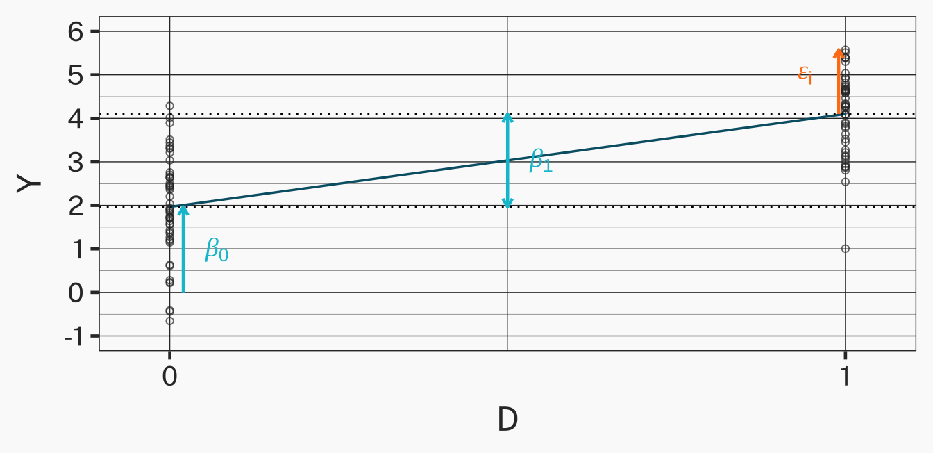
The simplest ATE estimator just plugs sample means into the identification formula. The OLS coefficient on \(D\) in the regression \(Y_i = \beta_0 + \beta_1 D_i + \varepsilon_i\) delivers the same number from a different starting point.
Start from the consistency identity for the observed outcome:
\[Y_i \;=\; Y_i(1) \cdot D_i \;+\; Y_i(0) \cdot (1 - D_i) \;=\; Y_i(0) \;+\; (Y_i(1) - Y_i(0))\, D_i.\]
Take conditional expectations given \(D_i\) in the population:
\[\mathbb{E}[Y_i \mid D_i] \;=\; \mathbb{E}[Y_i(0) \mid D_i] \;+\; \big(\mathbb{E}[Y_i(1) \mid D_i] - \mathbb{E}[Y_i(0) \mid D_i]\big) \cdot D_i.\]
Apply exchangeability (\(\{Y(1), Y(0)\} \perp\!\!\!\perp D\)): the conditional expectations on the right-hand side do not depend on \(D_i\), so \(\mathbb{E}[Y_i(0) \mid D_i] = \mathbb{E}[Y_i \mid D_i = 0]\) and \(\mathbb{E}[Y_i(1) - Y_i(0) \mid D_i] = ATE_{cs}\). Substituting:
\[\mathbb{E}[Y_i \mid D_i] \;=\; \underbrace{\mathbb{E}[Y_i \mid D_i = 0]}_{\beta_0} \;+\; \underbrace{ATE_{cs}}_{\beta_1}\, D_i.\]
So the population OLS slope \(\beta_1\) is exactly the causal ATE, and the intercept \(\beta_0\) is the marginal mean of the untreated potential outcome.
6.3.3.5 Residuals visualised, and OLS as SSR-minimisation
With a binary \(D\), the regression line connects two points: \((0, \beta_0)\) and \((1, \beta_0 + \beta_1)\). The deck visualises this on a 2-group scatter (slide “Residuals visualised”): each observation sits on either \(D = 0\) or \(D = 1\), the two horizontal mean lines are at heights \(\beta_0\) and \(\beta_0 + \beta_1\), the vertical gap between them is the slope \(\beta_1\), and each residual \(\varepsilon_i = Y_i - (\beta_0 + \beta_1 D_i)\) is the vertical distance from a point to its group mean. OLS literally fits two horizontal lines, one per group; the slope is the difference of their heights.
The sample estimator is the OLS minimiser:
\[\hat\beta_0,\; \hat\beta_1 \;=\; \arg\min_{\beta_0^*,\, \beta_1^*} \sum_{i=1}^n (Y_i - \beta_0^* - \beta_1^* D_i)^2.\]
Solving the first-order conditions yields the closed-form
\[\hat\beta_1 \;=\; \frac{\widehat{\text{Cov}}(Y_i, D_i)}{\widehat{\text{Var}}(D_i)}, \qquad \hat\beta_0 \;=\; \bar Y - \hat\beta_1 \bar D.\]
With binary \(D\), this is algebraically identical to the difference of group means — a useful sanity-check derivation. Under standard regularity conditions (Wooldridge 2010, ch. 4), OLS has three properties that justify treating it as the workhorse estimator for RCTs — developed in the next section.
6.3.4 Inference: standard errors, hypothesis tests, confidence intervals, bootstrap
Once \(\hat\beta_1\) is in hand, the next question is: how confident are we? Inference quantifies the sampling variability of the estimator.
6.3.4.1 OLS asymptotic properties
Under standard regularity conditions (Wooldridge 2010, ch. 4):
- Unbiasedness: \(\mathbb{E}[\hat\beta_1] = \beta_1\). Across hypothetical repeated random assignments, the estimator equals the true ATE on average.
- Consistency: \(\hat\beta_1 \xrightarrow{p} \beta_1\) as \(n \to \infty\). The estimator concentrates on the true value as the sample grows.
- Asymptotic normality: \(\sqrt{n}(\hat\beta_1 - \beta_1) \xrightarrow{d} \mathcal{N}(0, \sigma^2_{\beta_1})\). The sampling distribution is approximately normal in large samples, so standard \(t\)-tests and CIs apply.
Useful re-interpretation: OLS as moment matching. The OLS estimator solves the sample moment condition \(\frac{1}{n}\sum_i (Y_i - \beta_0 - \beta_1 D_i)(1, D_i)^\top = 0\). The same machinery returns in Session 06 (inverse-probability weighting estimates a different moment condition involving the propensity score) and Session 08 (double machine learning solves a Neyman-orthogonal moment condition robust to nuisance estimation). What changes from session to session is the moment condition; the estimating-equation framework is the constant.
6.3.4.2 Neyman vs. Fisher: what’s actually random?
In an RCT, who actually randomizes? The coin flip — not nature drawing from an infinite population. Standard CLT-based inference assumes the sample is one i.i.d. draw from a superpopulation; in an RCT, the only thing that is actually random is the treatment-assignment vector among the specific units in front of us. Two traditions answer this differently:
- Neyman (1923) — large-sample. Asks “how big is the average effect, and how precisely?” Tests the weak null \(\mathbb{E}[Y(1) - Y(0)] = 0\). Treats the potential outcomes as fixed; randomization is the source of variability; the sampling distribution of \(\hat\tau\) is recovered asymptotically: \(\sqrt{n}(\hat\tau - \tau) \xrightarrow{d} \mathcal{N}(0,\, V_N)\). Output: point estimate plus asymptotic SE plus CI. The variance \(V_N\) is conservatively estimated under treatment-effect heterogeneity (Neyman’s variance bound). Pros: closed-form CIs, scales to large \(n\), dominates textbooks. Cons: only valid asymptotically; conservative in small samples.
- Fisher (1925) — exact. Asks “could this difference be a coincidence under no effect for anyone?” Tests the sharp null \(H_0: Y_i(1) = Y_i(0)\) for every unit \(i\). Under \(H_0\), observed outcomes are fixed; the test-statistic distribution comes from re-shuffling treatment labels across all \(\binom{n}{n_1}\) permutations, giving an exact finite-sample p-value \(p = \frac{1}{|\mathcal{P}|}\sum_{\pi \in \mathcal{P}} \mathbf{1}\{|\hat\tau_\pi| \geq |\hat\tau_{\text{obs}}|\}\). Pros: no asymptotic approximation; works in tiny samples. Cons: tests a sharp (stronger) null; compute-intensive.
For the rest of this session, we ride with Neyman: closed-form HC SEs, t-tests, CIs. But the Fisher idea is not retired — its permutation logic returns next session as the engine behind A/B-test p-values in modern tech-company experimentation platforms (especially for the small-sample regime where asymptotic approximations are unreliable). For typical \(n \gtrsim 1000\), Neyman and Fisher p-values agree to several decimal places; Exercise 2 verifies this empirically.
6.3.4.3 The heteroskedasticity-robust standard error
Under asymptotic normality, the variance of \(\hat\beta_1\) takes the sandwich form:
\[\text{Var}(\hat\beta_1) \;=\; \frac{\mathbb{E}[\varepsilon_i^2 (D_i - \mathbb{E}[D_i])^2]}{n \cdot (\text{Var}(D_i))^2}.\]
The sample analogue replaces population moments with sample moments and the unobservable \(\varepsilon_i\) with the OLS residuals \(\hat\varepsilon_i = Y_i - \hat\beta_0 - \hat\beta_1 D_i\):
\[\widehat{\text{Var}}(\hat\beta_1) \;=\; \frac{\sum_i \hat\varepsilon_i^2 (D_i - \bar D)^2}{\big[\sum_i (D_i - \bar D)^2\big]^2}, \qquad se(\hat\beta_1) \;=\; \sqrt{\widehat{\text{Var}}(\hat\beta_1)}.\]
This is the HC0 sandwich estimator. R’s sandwich::vcovHC(fit, type = "HC1") and Python’s cov_type="HC1" apply a small-sample correction factor \(n/(n-k)\). Many textbooks (and the legacy slide deck) called this the “asymptotic variance” — a label that obscures the distinction from the homoskedastic version. The classical homoskedastic SE simplifies to \(\sigma^2_\varepsilon / (n \cdot \text{Var}(D))\), which assumes the residual variance does not vary with \(D\). In an RCT with two arms, residual variances are virtually always different across arms (treatment and control populations behave differently around their means), so always default to HC.
6.3.4.4 Reading the t-distribution
The standardised statistic with known \(sd\) is normal; with the estimated \(se\) it is \(t\)-distributed with \(df = n - 2\) for the binary-treatment regression:
\[z_1 = \frac{\hat\beta_1 - \beta_1}{sd(\hat\beta_1)} \xrightarrow{d} \mathcal{N}(0, 1) \qquad \text{vs.} \qquad t_1 = \frac{\hat\beta_1 - \beta_1}{se(\hat\beta_1)} \sim t_{n-2}.\]
The slide deck plots two t-densities side by side — left for a two-sided test at \(\alpha = 5\%\) with critical values \(\pm 1.96\) and 2.5% area in each tail; right for a one-sided test at \(\alpha = 5\%\) with critical value \(1.65\) and the full 5% in one tail. The blue shaded area is the rejection region: when the observed t-statistic lands there under the null, we reject. For any \(n \gtrsim 30\) the t-distribution is indistinguishable from \(\mathcal{N}(0,1)\) in a plot, but we still write t-distribution because the SE is estimated, not known.
6.3.4.5 Hypothesis testing — the four-step procedure
Step 1. State the null and alternative:
- Two-sided (undirected): \(H_0: \beta_1 = 0\) vs. \(H_1: \beta_1 \neq 0\).
- One-sided (directed, positive): \(H_0: \beta_1 \leq 0\) vs. \(H_1: \beta_1 > 0\).
- One-sided (directed, negative): \(H_0: \beta_1 \geq 0\) vs. \(H_1: \beta_1 < 0\).
Two-sided is the workhorse: reject if the data are far from zero in either direction. One-sided is appropriate only when directional theory rules out one tail before seeing the data — which is rare and usually a red flag for HARKing if applied post hoc.
Step 2. Set the significance level \(\alpha\) — the maximally accepted type I error rate (false rejections under a true null). \(\alpha = 0.05\) means at most a 5% rate of false rejections in repeated samples; conventional alternatives are \(\alpha = 0.01\) and \(\alpha = 0.10\).
Step 3. Compute the critical value \(c\) as a quantile of the \(t\)-distribution under \(H_0\). Two-sided \(\alpha = 0.05\), \(df = 998\): \(c = t_{0.025,\,998} \approx 1.96\). One-sided \(\alpha = 0.05\), \(df = 998\): \(c = t_{0.05,\,998} \approx 1.65\).
Step 4. Compute the test statistic and p-value and apply the decision rule:
\[t_1 \;=\; \frac{\hat\beta_1 - 0}{se(\hat\beta_1)}, \qquad p \;=\; P(|A| \geq |t_1|) \text{ for } A \sim t_{n-2}.\]
Reject \(H_0\) if \(|t_1| > c\), equivalently \(p < \alpha\). Worked example with \(\hat\beta_1 = 0.30\), \(se = 0.05\): \(t = 6.0\), far outside \(\pm 1.96\), so reject. Two-sided p-value \(p = 2 \cdot \Phi(-6.0) < 10^{-9}\). Note: small \(p\) does not mean the null is unlikely; it means the data are unlikely given the null. Misreading this is the classic prosecutor’s fallacy.
6.3.4.6 Confidence intervals
A \((1 - \alpha)\) confidence interval is the range of values \(\beta_1^*\) for which the corresponding null \(H_0: \beta_1 = \beta_1^*\) would not be rejected at level \(\alpha\):
\[CI \;=\; \hat\beta_1 \;\pm\; c \cdot se(\hat\beta_1).\]
With \(\hat\beta_1 = 0.30\), \(se = 0.05\), \(c = 1.96\): \(CI = [0.202,\; 0.398]\). The CI excludes zero — the same conclusion as the t-test, just expressed as a range. Frequentist interpretation: across hypothetical repeated samples, \((1 - \alpha)\) of the constructed CIs would cover the true \(\beta_1\). Any single realised interval either covers or doesn’t; no probability statement attaches to a specific CI.
One-sided CI: \([\hat\beta_1 - c \cdot se(\hat\beta_1),\, \infty)\) (upper open) or \((-\infty,\, \hat\beta_1 + c \cdot se(\hat\beta_1)]\) (lower open). Used when only one direction of the parameter is substantively meaningful.
6.3.4.7 Common misinterpretations of \(\alpha\) and CIs — and where the intuitive reading actually lives
The frequentist machinery is precise but not intuitive. Students, reviewers, and journalists routinely misread it:
| What people want it to mean | What it actually means |
|---|---|
| “\(p = 0.03\) means there’s a 3% chance the null is true.” | \(p\) is the probability of data this extreme given \(H_0\) is true, \(P(\text{data} \mid H_0)\). |
| “There’s a 95% chance the true \(\beta_1\) lies in this CI.” | Across hypothetical re-samples, 95% of the constructed intervals cover \(\beta_1\). Any single realised interval either covers or doesn’t. |
| “\(\alpha = 0.05\) is the probability I’m wrong.” | \(\alpha\) is the long-run type I error rate of the procedure. |
| “A non-significant result means \(H_0\) is true.” | Non-significant ≠ “no effect.” Only “no detectable effect at this \(n\) and \(\alpha\).” |
All the left-column readings are probability statements about hypotheses or parameters given data, \(P(H_0 \mid \text{data})\) or \(P(\beta_1 \in CI \mid \text{data})\). Frequentist inference cannot deliver these; it makes statements about the procedure, not the parameter.
The intuitive readings are legitimate — under Bayesian inference. With a prior on \(\beta_1\), the posterior \(P(\beta_1 \mid \text{data})\) supports direct statements like “there’s a 95% chance \(\beta_1 \in [0.20,\, 0.40]\)”. That’s the credible interval, the Bayesian counterpart of the frequentist CI. Bayesian A/B testing and credible intervals are formally introduced in Session 5: Online A/B Testing, alongside CUPED and stratified A/B testing.
6.3.4.8 R-squared — diagnostic, not destination
For any regression, \(R^2 = 1 - \frac{SSR}{SST}\) where \(SSR = \sum_i (Y_i - \hat Y_i)^2\) and \(SST = \sum_i (Y_i - \bar Y)^2\). In the special case of a single binary treatment, \(R^2\) collapses to the squared Pearson correlation between \(Y\) and \(D\):
\[R^2 \;=\; r^2 \;=\; \left( \frac{\sum_i (Y_i - \bar Y)(D_i - \bar D)}{\sqrt{\sum_i (Y_i - \bar Y)^2 \cdot \sum_i (D_i - \bar D)^2}} \right)^{\!2}.\]
In a causal-inference context, \(R^2\) is largely diagnostic — a randomized treatment effect can be small relative to total \(Y\)-variance (low \(R^2\)) yet perfectly identified and statistically significant. Conversely, a regression with high \(R^2\) can still be confounded if it includes the wrong covariates. Don’t optimise for \(R^2\) in causal work — optimise for unbiased identification.
6.3.4.9 Job Corps via OLS with HC-robust SEs
The standard reporting workflow on the Job Corps RCT is lm() (or smf.ols) plus sandwich::vcovHC (or cov_type="HC1"), with modelsummary for a publication-ready table. Both tracks produce numerically identical (within rounding) point estimates and SEs.
library(sandwich)
library(modelsummary)

jc <- read_csv(here("materials/data/jc.csv"), show_col_types = FALSE)
ols_jc <- lm(earny4 ~ assignment, data = jc)

modelsummary(ols_jc,
  vcov = sandwich::vcovHC,
  estimate = "{estimate} (se = {std.error}, t = {statistic}){stars}",
  statistic = "p = {p.value}, CI = [{conf.low}, {conf.high}]",
  stars = TRUE,
  gof_map = c("r.squared", "nobs"),
output = "markdown")| (Intercept) | 197.926 (se = 3.073, t = 64.416)*** |
| p = <0.001, CI = [191.903, 203.949] | |
| assignment | 16.055 (se = 4.074, t = 3.941)*** |
| p = <0.001, CI = [8.069, 24.041] | |
| R2 | 0.002 |
| Num.Obs. | 9240 |
import pandas as pd
import statsmodels.formula.api as smf
jc = pd.read_csv("../../materials/data/jc.csv")
ols_jc = smf.ols("earny4 ~ assignment", data=jc).fit(cov_type="HC1")
print(ols_jc.summary().tables[1])
==============================================================================
coef std err z P>|z| [0.025 0.975]
------------------------------------------------------------------------------
Intercept 197.9258 3.072 64.427 0.000 191.905 203.947
assignment 16.0551 4.074 3.941 0.000 8.071 24.039
==============================================================================The reported coefficient on assignment is the ATE on weekly earnings; the 95% CI excludes zero, so we reject the null of no effect at \(\alpha = 5\%\). This is the analysis we’d write up in a paper.
6.3.4.10 Bootstrap
A third route to inference — alongside Neyman’s analytical SE and Fisher’s randomization test — is the non-parametric bootstrap (Huber 2023): treat the empirical distribution as if it were the population, draw \(B\) resamples of size \(n\) with replacement, recompute \(\hat\beta_1^{(b)}\) on each, and take the empirical SD across replicates as the SE:
\[se_{\text{boot}}(\hat\beta_1) \;=\; \sqrt{\tfrac{1}{B - 1} \sum_{b=1}^{B} (\hat\beta_1^{(b)} - \bar{\hat\beta_1})^2}.\]
Standard practice is \(B = 1{,}999\) (just below 2000 to make percentile-rank computations clean). For OLS with HC SEs the bootstrap is essentially redundant — it estimates the same quantity — but for non-standard estimators (kernel regression, propensity-score-weighted, doubly-robust) where the analytical SE is hard to derive, the bootstrap is the workhorse. R: boot::boot(). Python: scipy.stats.bootstrap (SciPy ≥ 1.7) or hand-rolled numpy.random.choice with replacement.
When bootstrap > HC-robust: small \(n\), heavy-tailed \(\varepsilon\), clustered or dependent data, or non-smooth statistics (medians, quantiles, ratios). Otherwise HC1 is faster and equally honest.
6.3.5 Multivalued and continuous treatments
OLS extends naturally beyond the binary case in two directions.
6.3.5.1 Multivalued (categorical) treatments
Suppose \(D\) takes \(J + 1\) values \(\{0, 1, \ldots, J\}\) (e.g., dosage levels, marketing-channel arms, multi-arm A/B tests). The independence assumption generalises to all levels: \(\{Y(0), Y(1), \ldots, Y(J)\} \perp\!\!\!\perp D\). Encode each non-baseline level as a binary dummy \(D_{i,j} = \mathbf{1}\{D_i = j\}\) and run OLS with \(D = 0\) as the reference category:
\[\mathbb{E}[Y_i \mid D_i] \;=\; \beta_0 \;+\; \beta_1 D_{i,1} \;+\; \cdots \;+\; \beta_J D_{i,J}.\]
Each \(\beta_j = \mathbb{E}[Y(j) - Y(0)]\) is the ATE of arm \(j\) vs. the reference arm. Pairwise contrasts (arm \(j\) vs. arm \(k\)) are recovered as \(\beta_j - \beta_k\). Software handles this automatically: in R, factor(D) and lm() produce the full set of dummies; in Python, smf.ols("Y ~ C(D)", data=df) does the same. To get an ATE between two non-baseline levels, take the difference of coefficients (or re-parameterize with a different reference).
6.3.5.2 Continuous treatments
Suppose \(D\) is continuous (e.g., dollars of advertising spend, price level, dosage). The randomization assumption now reads \(Y(d) \perp\!\!\!\perp D\) for every \(d\) in the support. The estimand is the marginal effect
\[ATE(d) \;=\; \frac{\partial \mathbb{E}[Y \mid D = d]}{\partial D}.\]
Two strategies:
- Discretise. Bin \(D\) into a small number of categories (quartiles, expert-defined breakpoints) and apply the multivalued-treatment recipe above. Loses information but easy to communicate.
- Linear regression with \(D\) continuous. Fit \(Y = \beta_0 + \beta_1 D + \varepsilon\). Then \(ATE(d) = \beta_1\), a constant marginal effect.
The constant-marginal-effect assumption is restrictive; the slides illustrate the difference visually with a linear DGP (constant slope) and a non-linear DGP (slope varying with \(D\)). To allow non-linearity, add a polynomial term:
\[Y = \beta_0 + \beta_1 D + \beta_2 D^2 + \varepsilon \quad \Rightarrow \quad ATE(d) = \beta_1 + 2\beta_2 d,\]
a marginal effect that varies with the dose. More flexibly, kernel regression estimates \(\widehat{\mathbb{E}}[Y \mid D = d]\) as a locally weighted average of nearby \(Y_i\) values, with a bandwidth parameter controlling “close” — R: np::npreg; Python: statsmodels.nonparametric.kernel_regression.KernelReg. Splines are a third option (R: splines::ns; Python: patsy.bs). The marginal effect at any \(d\) is just the slope of the fitted curve there.
Flexible nuisance estimators like splines and kernel regression are the workhorses of modern double machine learning (Session 08), where they appear inside an orthogonal moment condition that makes the resulting causal estimator robust to the specific nuisance choice. Session 04 keeps things simple: with random assignment, even a misspecified linear model still recovers the average marginal effect under conditions on the moment of \(D\).
6.3.6 Including covariates: variance reduction, not bias correction
Suppose we also observe pre-treatment covariates \(X_{i,1}, \ldots, X_{i,K}\) (e.g., age, prior-period spend, app version). Under randomization, \(D \perp X\), so adding pre-treatment covariates does not change the population value of \(\hat\beta_1\) — it cannot fix bias that does not exist. What it does change is precision: the residual variance shrinks, and so does \(se(\hat\beta_1)\).
\[Y_i \;=\; \underbrace{\hat\beta_0 + \hat\beta_1 D_i + \hat\beta_{X_1} X_{i,1} + \ldots + \hat\beta_{X_K} X_{i,K}}_{\widehat{\mathbb{E}}[Y_i \mid D_i, X_i]} \;+\; \hat\varepsilon_i.\]
The covariates explain part of the variation in \(Y\) that was previously residual: \(R^2 \uparrow,\ \widehat{\text{Var}}(\hat\varepsilon)/\widehat{\text{Var}}(Y) \downarrow,\ se(\hat\beta_1) \downarrow\). This is the only legitimate role of covariates under randomization. Confounding adjustment is not on the table because there is no confounding to adjust for — \(D\) is independent of \(X\) by construction. Compare with Session 06, where \(D\) is not random and covariates serve a fundamentally different purpose (de-confounding via backdoor adjustment, IPW, or matching). Same regression syntax, two fundamentally different statistical roles.
6.3.6.1 Freedman (2008) and the Lin (2013) fix
5 pointed out a subtle issue: in finite samples, the additive covariate-adjusted OLS estimator \(Y \sim D + X\) has small-sample bias whenever the treatment effect varies with \(X\) (treatment-effect heterogeneity).
Why? \(Y \sim D + X\) assumes one effect \(\beta_1\) for everyone. With true heterogeneity \(\tau(X)\), OLS instead recovers a \(\widehat{\text{Var}}(D \mid X)\)-weighted average of conditional ATEs — and finite-sample imbalance in \(X\) tilts those weights off the marginal density that defines the ATE. The bias is asymptotically negligible but can matter at typical RCT sample sizes.
4 proposed the canonical fix: regress \(Y\) on \(D\), mean-centred \(X\), and the interaction \(D \cdot (X - \bar X)\):
\[Y_i \;=\; \beta_0 \;+\; \beta_1 D_i \;+\; \boldsymbol{\gamma}^\top (X_i - \bar X) \;+\; \boldsymbol{\delta}^\top D_i (X_i - \bar X) \;+\; \varepsilon_i.\]
The Lin estimator is unbiased for the ATE in finite samples, allows treatment-effect heterogeneity, and typically attains lower variance than both the unadjusted and the additive-adjusted estimators. Mean-centring \(X\) is critical: it ensures that \(\hat\beta_1\) continues to read as the average treatment effect (rather than the conditional effect at \(X = 0\)). Modern best-practice default for covariate adjustment in randomized experiments.
Two practical warnings:
- Pre-specify the covariates in the analysis plan. Otherwise covariate inclusion becomes a data-mining exercise: trying many specifications until \(\hat\beta_1\) becomes “significant” inflates the type-I error rate, no matter how innocent the intent. Tech A/B-testing platforms typically lock the analysis specification before the experiment is launched.
- Never include post-treatment covariates — the pre- vs. post-treatment lesson, with the DAGs to make it visceral.
6.3.6.2 Pre-treatment vs. post-treatment covariates — the DAG view
The slides put two DAGs side by side. Pre-treatment covariates are parents of \(Y\) but exogenous to \(D\): they share no causal ancestry with the treatment. Adding them to the regression reduces residual variance without changing the expectation of \(\hat\beta_1\) — safe, and the basis for variance reduction.
Post-treatment covariates are descendants of \(D\) in the causal graph. Conditioning on them does two harmful things at once:
- Mediator-blocking: closes part of \(D \to X \to Y\) — you would estimate the direct effect of \(D\) on \(Y\) rather than the total effect, which is rarely what we actually want.
- Collider-opening: when \(X\) shares an unobserved parent \(U\) with \(Y\), conditioning on \(X\) opens the path \(D \to X \leftarrow U \to Y\), re-introducing confounding (back to Session 02’s collider lesson).
Attaching package: 'ggdag'The following object is masked from 'package:stats':
filter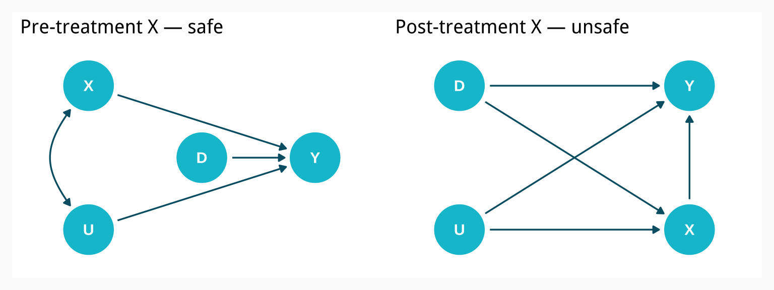
Practical heuristic: if the variable was measured during or after the treatment period, treat it as suspect. Variables measured before random assignment was implemented are safe candidates for variance reduction; everything else needs an explicit causal-graph defence. The strict rule from 4 and the broader RCT literature: pre-specify the covariate list in the analysis plan, and never edit it after seeing the outcome. Exercise 4 makes the collider trap concrete by including a deliberately mis-specified post-treatment covariate and watching the resulting bias.
6.3.6.3 Worked example: coffee-leaflet RCT
The slides apply the full covariate-adjusted workflow to coffeeleaflet.csv — 522 university students randomly assigned to receive (or not) an environmental-impact leaflet about coffee. Outcome: awarewaste (waste-awareness scale); covariates: mumedu (mother’s education) and sex (both pre-treatment demographics). The coefficient on treatment is the ATE of the leaflet on waste-awareness, with HC-robust SE; the mumedu and sex coefficients are absorbed-variance covariates and should not be interpreted as ATEs of those variables (they were not randomized). The full code is on the slide; we revisit a structurally identical pattern in Exercise 4 with the in-app feature data.
6.4 Coding Lab
Five exercises, increasing in difficulty and total budget ≈ 135 minutes:
| # | Topic | Slide stack | Time |
|---|---|---|---|
| 1 | Causal vs. associational ATE; bias decomposition (Christmas/socks) | Randomization | ~25 min |
| 2 | Manual SE/CI/HT, OLS verification, bootstrap, Fisher randomization test (in-app feature) | Identification + Inference | ~40 min |
| 3 | Variance reduction via blocked random assignment | Randomization → Inference | ~20 min |
| 4 | Lin (2013) covariate adjustment + post-treatment collider trap | Extensions | ~30 min |
| 5 | Multivalued (3-arm wexpect) + continuous (kernel regression on marketing) | Extensions | ~20 min |
All exercises are bilingual: every R chunk has a Python equivalent in a panel-tabset.
6.4.1 Exercise 1 — Causal vs. associational ATE on Christmas/socks data (~25 min)
You are the owner of an online marketplace company that small and medium-sized businesses use to sell products. The businesses act autonomously regarding prices, advertising, and so on. Because your revenue depends on the prosperity of these businesses, you want to support them by offering guidance about when to run sales campaigns. From a business perspective, a price drop is beneficial when the increase in number of sold units compensates for the lower price, so the key quantity is the causal effect of a sales campaign on units sold. For simplicity, focus on a single product category — socks — in the weeks leading up to Christmas.
Data (materials/data/xmas_sales.csv, 2,000 store-week observations):
store— unique store identifierweeks_to_xmas— weeks until Christmas (4 = four weeks before, 0 = Christmas week)avg_week_sales— store-level historical average of weekly sales (a measure of business size)is_on_sale— \(D_i \in \{0, 1\}\), indicator for whether the store ran a price reduction that weekweekly_amount_sold— \(Y_i\), the outcome of interest
6.4.1.1 Scaffold
Six steps; load + inspect + box plot + naive ATE on the realistic data, then switch to the toy sales_unreal.csv with both potential outcomes observed to compute the causal ATE and decompose the bias.
library(tidyverse); library(here)

# Step 1: load realistic data, coerce is_on_sale to logical, glimpse
sales <- # ___ YOUR CODE: read_csv(here("materials/data/xmas_sales.csv"), ...)

# Step 2: box plot of weekly_amount_sold by is_on_sale.

# Step 3: naive associational ATE
y1_mean <- # ___ YOUR CODE
y0_mean <- # ___ YOUR CODE
naive_ate <- # ___ YOUR CODE: y1_mean - y0_mean   # ~ 78

# Step 4: switch to the toy counterfactual file (both Y(0) and Y(1) observed)
sales_unreal <- read_csv(here("materials/data/sales_unreal.csv"), show_col_types = FALSE)
ATE_causal <- # ___ YOUR CODE: mean(y1 - y0)       # ~ 15

# Step 5: decompose the associational ATE into (causal + confounding + heterogeneity).
# Using the bias-decomposition gold equation:
#   ATE_as = ATE_cs + E[Y(0)|D=1] - E[Y(0)|D=0]  +  (1 - E[D]) * (ATT - ATU)
BIAS_conf <- # ___ YOUR CODE
ATT       <- # ___ YOUR CODE: mean(y1 - y0 | treated)
ATU       <- # ___ YOUR CODE
BIAS_het  <- # ___ YOUR CODE
# Confirm: ATE_causal + BIAS_conf + BIAS_het == naive_ate_on_toy
import pandas as pd
# Step 1
sales = # ___ YOUR CODE: pd.read_csv("../../materials/data/xmas_sales.csv")
# Step 3: naive ATE
y1_mean = # ___ YOUR CODE
y0_mean = # ___ YOUR CODE
naive_ate = # ___ YOUR CODE # ~ 78
# Step 4: switch to sales_unreal.csv
sales_unreal = pd.read_csv("../../materials/data/sales_unreal.csv")
ATE_causal = # ___ YOUR CODE # ~ 15
# Step 5: confounding + heterogeneity bias decomposition.
BIAS_conf = # ___ YOUR CODE
ATT = # ___ YOUR CODE
ATU = # ___ YOUR CODE
BIAS_het = # ___ YOUR CODE
TipShow solution
6.4.1.2 Step 1 — Load the data and inspect
library(tidyverse)
sales <- read_csv(here("materials/data/xmas_sales.csv"), show_col_types = FALSE) |>
  mutate(is_on_sale = as.logical(is_on_sale))
glimpse(sales)
Rows: 2,000
Columns: 5
$ store <dbl> 1, 1, 1, 1, 2, 2, 2, 2, 3, 3, 3, 3, 4, 4, 4, 4, 5, …
$ weeks_to_xmas <dbl> 3, 2, 1, 0, 3, 2, 1, 0, 3, 2, 1, 0, 3, 2, 1, 0, 3, …
$ avg_week_sales <dbl> 12.98, 12.98, 12.98, 12.98, 19.92, 19.92, 19.92, 19…
$ is_on_sale <lgl> TRUE, TRUE, TRUE, FALSE, FALSE, FALSE, FALSE, FALSE…
$ weekly_amount_sold <dbl> 219.60, 184.70, 145.75, 102.45, 103.22, 53.73, 13.8…import pandas as pd
sales = pd.read_csv("../../materials/data/xmas_sales.csv")
sales["is_on_sale"] = sales["is_on_sale"].astype(bool)
print(sales.head()); print(sales.shape) store weeks_to_xmas avg_week_sales is_on_sale weekly_amount_sold
0 1 3 12.98 True 219.60
1 1 2 12.98 True 184.70
2 1 1 12.98 True 145.75
3 1 0 12.98 False 102.45
4 2 3 19.92 False 103.22
(2000, 5)6.4.1.3 Step 2 — Box plot: \(Y\) by \(D\)
ggplot(sales, aes(x = is_on_sale, y = weekly_amount_sold, fill = is_on_sale)) +
  geom_boxplot(alpha = 0.7) +
  scale_fill_manual(values = c("FALSE" = "#005e73", "TRUE" = "#FF7E15")) +
  labs(x = "On sale (D)", y = "Weekly amount sold (Y)") +
  theme(legend.position = "none")
import matplotlib.pyplot as plt
fig, ax = plt.subplots(figsize=(5, 3.5))
sales.boxplot(column="weekly_amount_sold", by="is_on_sale", ax=ax,
              boxprops=dict(color="#005e73"), medianprops=dict(color="#FF7E15"))
ax.set_xlabel("On sale (D)"); ax.set_ylabel("Weekly amount sold (Y)")
ax.set_title(""); plt.suptitle("")
plt.tight_layout(); plt.show()
Stores that dropped their prices sell more. The difference looks very large.
6.4.1.4 Step 3 — Compute the naive (associational) ATE
y1_mean <- mean(sales$weekly_amount_sold[sales$is_on_sale])
y0_mean <- mean(sales$weekly_amount_sold[!sales$is_on_sale])
c("Avg. on sale (D=1)"        = y1_mean,
  "Avg. not on sale (D=0)"    = y0_mean,
  "Naive ATE (associational)" = y1_mean - y0_mean)
Avg. on sale (D=1) Avg. not on sale (D=0) Naive ATE (associational)
141.03383 63.07972 77.95410 y1_mean = sales.loc[sales.is_on_sale, "weekly_amount_sold"].mean()
y0_mean = sales.loc[~sales.is_on_sale, "weekly_amount_sold"].mean()
print({"Avg. on sale (D=1)": round(y1_mean, 2),
"Avg. not on sale (D=0)": round(y0_mean, 2),
"Naive ATE (associational)": round(y1_mean - y0_mean, 2)}){'Avg. on sale (D=1)': np.float64(141.03), 'Avg. not on sale (D=0)': np.float64(63.08), 'Naive ATE (associational)': np.float64(77.95)}The naive estimate is around 78 units — larger than the average outcome of stores that did not run a sale (\(\approx 63\)). That should set off an alarm: a simple comparison is very unlikely to give a valid causal answer here. Hold on to the number 78 — in Step 4 we will reproduce the same associational ATE on a toy dataset where, because we observe both potential outcomes, we can decompose it into a causal piece and two bias pieces.
Question. What explanations can you think of that distort the relationship between treatment and outcome? Think back to Session 02.
Answer
Two confounders — common causes of both treatment and outcome:
- Business size (
avg_week_sales). Larger businesses are both more likely to run sales campaigns and sell more units, on or off sale. This is a fork: \(\text{size} \to \text{is\_on\_sale}\) and \(\text{size} \to \text{weekly\_amount\_sold}\). - Time to Christmas (
weeks_to_xmas). Stores tend to run sales campaigns closer to Christmas, when customers are buying anyway.
A scatter plot of weekly_amount_sold vs. avg_week_sales, coloured by is_on_sale, makes the size effect visible: the orange (on-sale) points are concentrated among the larger-business observations.
6.4.1.5 Step 4 — Switch to the unrealistic full-counterfactual scenario
In the realistic data, we observe one outcome per store — the fundamental problem of causal inference. To make the bias decomposition fully visible, we now switch to a small toy dataset where, by simulation, we observe both potential outcomes for every unit.
The data in sales_unreal.csv has 6 stores with columns i, y0, y1, t, x, y, te (where te = y1 - y0 is the individual treatment effect).
sales_unreal <- read_csv(here("materials/data/sales_unreal.csv"), show_col_types = FALSE)
sales_unreal
# A tibble: 6 × 7
i y0 y1 t x y te
<dbl> <dbl> <dbl> <dbl> <dbl> <dbl> <dbl>
1 1 40 45 0 0 40 5
2 2 60 67 0 0 60 7
3 3 89 98 0 1 89 9
4 4 100 120 1 1 120 20
5 5 120 143 1 1 143 23
6 6 134 160 1 1 160 26sales_unreal = pd.read_csv("../../materials/data/sales_unreal.csv")
sales_unreal i y0 y1 t x y te
0 1 40 45 0 0 40 5
1 2 60 67 0 0 60 7
2 3 89 98 0 1 89 9
3 4 100 120 1 1 120 20
4 5 120 143 1 1 143 23
5 6 134 160 1 1 160 26The causal ATE is just the average of the individual treatment effects:
ATE_causal <- mean(sales_unreal$y1 - sales_unreal$y0)
ATE_causal
[1] 15ATE_causal = (sales_unreal["y1"] - sales_unreal["y0"]).mean()
print(ATE_causal)15.0The true causal ATE is 15 — five times smaller than the 78 we computed on the realistic data. By contrast, the associational ATE on this same toy data (averaging the observed y separately by t) is exactly 78, matching what we saw in Step 3. The toy is calibrated so that the observed group means coincide with the realistic data (\(\bar y \mid t=1 = 141\), \(\bar y \mid t=0 = 63\)); the only thing the toy adds is the second potential outcome, which lets us decompose where the 78 - 15 = 63 unit gap comes from.
6.4.1.6 Step 5 — Decompose the bias
Use the bias-decomposition gold equation to break the gap between \(ATE_{as}\) and \(ATE_{cs}\) into a confounding-bias term and a heterogeneity-bias term:
\[ATE_{as} \;=\; ATE_{cs} \;+\; \underbrace{\mathbb{E}[Y(0) \mid D=1] - \mathbb{E}[Y(0) \mid D=0]}_{\text{Conf. bias}} \;+\; \underbrace{(1 - \mathbb{E}[D]) (\text{ATT} - \text{ATU})}_{\text{Het. bias}}.\]
treat <- sales_unreal$t == 1
ctrl  <- sales_unreal$t == 0

ATE_causal <- mean(sales_unreal$y1 - sales_unreal$y0)
BIAS_conf  <- mean(sales_unreal$y0[treat]) - mean(sales_unreal$y0[ctrl])
ATT <- mean(sales_unreal$y1[treat] - sales_unreal$y0[treat])
ATU <- mean(sales_unreal$y1[ctrl]  - sales_unreal$y0[ctrl])
BIAS_het   <- (1 - mean(sales_unreal$t)) * (ATT - ATU)
ATE_assoc  <- ATE_causal + BIAS_conf + BIAS_het

c("Causal ATE"        = ATE_causal,
  "Confounding Bias"  = BIAS_conf,
  "Heterogeneity Bias"= BIAS_het,
  "Associational ATE" = ATE_assoc)
Causal ATE Confounding Bias Heterogeneity Bias Associational ATE
15 55 8 78 treat = sales_unreal["t"] == 1
ctrl = sales_unreal["t"] == 0
ATE_causal = (sales_unreal["y1"] - sales_unreal["y0"]).mean()
BIAS_conf = sales_unreal.loc[treat, "y0"].mean() - sales_unreal.loc[ctrl, "y0"].mean()
ATT = (sales_unreal.loc[treat, "y1"] - sales_unreal.loc[treat, "y0"]).mean()
ATU = (sales_unreal.loc[ctrl, "y1"] - sales_unreal.loc[ctrl, "y0"]).mean()
BIAS_het = (1 - sales_unreal["t"].mean()) * (ATT - ATU)
ATE_assoc = ATE_causal + BIAS_conf + BIAS_het
print({"Causal ATE": round(ATE_causal, 2),
"Confounding Bias": round(BIAS_conf, 2),
"Heterogeneity Bias": round(BIAS_het, 2),
"Associational ATE": round(ATE_assoc, 2)}){'Causal ATE': np.float64(15.0), 'Confounding Bias': np.float64(55.0), 'Heterogeneity Bias': np.float64(8.0), 'Associational ATE': np.float64(78.0)}6.4.1.7 Step 6 — Reflection
What did we learn?
Reading the table from Step 5: causal ATE = 15, confounding bias = 55, heterogeneity bias = 8, summing to the associational ATE = 78. The confounding bias dominates by a factor of roughly seven — businesses that adopt the price promotion have systematically higher baseline (untreated) sales than those that do not (mean \(Y(0) \mid D=1 = 118\) vs. \(\mathbb{E}[Y(0) \mid D=0] = 63\)). Heterogeneity plays a smaller role: treated stores benefit more from a sale than control stores would have (\(\text{ATT} = 23\) vs. \(\text{ATU} = 7\)), but it accounts for only one-tenth of the gap.
The realistic dataset shows the same confounding pattern in the avg_week_sales covariate: large businesses run sales more often and sell more units, on or off sale. The naive estimate of 78 is overwhelmingly driven by who gets treated, not by what the treatment does.
The cure that the rest of this session studies: if we had randomly assigned the price reduction to a subset of stores, both bias terms would be exactly zero in expectation, and the simple mean comparison would recover \(ATE_{cs}\). Without randomization, we need either an adjustment strategy (Session 06) or an instrument (Session 07).
6.4.2 Exercise 2 — Manual estimation, OLS, bootstrap, randomization inference (~40 min)
You are part of the business-analytics team at a software company. Your team rolled out a new in-app feature to a randomly chosen subset of users (random assignment was implemented by hashing the IP address). Your task: estimate the average effect of the feature on daily time spent in the app, and quantify uncertainty around the estimate. The exercise walks through the manual mechanics — group means, standard deviations, standard errors, confidence intervals, hypothesis test — verifies all of it via a single lm() / smf.ols() call, and finishes by reproducing the SE two more ways: a non-parametric bootstrap (the bootstrap) and a Fisher-style randomization test (Neyman vs. Fisher).
Data (materials/data/new_feature.csv, 1,000 users):
user_id— user identifiernew_feature— \(D_i \in \{0, 1\}\), indicator for whether the user got the new featuretime_spent— \(Y_i\), daily minutes spent in the app
6.4.2.1 Scaffold
Manual mechanics first; then verify via one lm() / smf.ols() call; then reproduce the SE two more ways (bootstrap, Fisher randomization test).
library(tidyverse); library(here)

df <- read_csv(here("materials/data/new_feature.csv"), show_col_types = FALSE)

# Step 2: group-specific means; naive ATE = mean(treated) - mean(control)
group_means <- # ___ YOUR CODE: df |> group_by(new_feature) |> summarise(mean_time_spent = mean(time_spent))
naive_ate   <- # ___ YOUR CODE

# Step 3: within-group SDs and the SE for the difference in means
#   SE(diff) = sqrt(s1^2/n1 + s0^2/n0)
sd_treated <- # ___ YOUR CODE
sd_control <- # ___ YOUR CODE
n_treated  <- sum(df$new_feature == 1); n_control <- sum(df$new_feature == 0)
se_diff    <- # ___ YOUR CODE: sqrt(sd_treated^2/n_treated + sd_control^2/n_control)

# Step 4: 95% CI and a two-sided t-test
ci         <- # ___ YOUR CODE: naive_ate ± 1.96 * se_diff
t_stat     <- # ___ YOUR CODE
p_value    <- # ___ YOUR CODE

# Step 5: verify everything via lm() with HC-robust SE
library(estimatr)
fit_lm <- # ___ YOUR CODE: lm_robust(time_spent ~ new_feature, data = df, se_type = "HC1")
summary(fit_lm)

# Step 6: non-parametric bootstrap of the ATE, B = 1000 reps
set.seed(2026)
boot_atehs <- # ___ YOUR CODE: replicate(1000, mean of treated minus control on a resample)
se_boot    <- sd(boot_atehs)

# Step 7: Fisher randomization test, reshuffling D under H_0: tau = 0
ate_perm <- # ___ YOUR CODE: replicate(1000, mean diff after random permutation of D)
p_fisher <- # ___ YOUR CODE: 2-sided rate at which |ate_perm| >= |naive_ate|
import numpy as np, pandas as pd
import statsmodels.api as sm
import statsmodels.formula.api as smf
df = pd.read_csv("../../materials/data/new_feature.csv")
# Step 2: group means + naive ATE
group_means = # ___ YOUR CODE
naive_ate = # ___ YOUR CODE
# Step 3-4: SDs, SE for diff of means, CI, t-test
sd_treated = # ___ YOUR CODE
sd_control = # ___ YOUR CODE
n_t = (df.new_feature == 1).sum(); n_c = (df.new_feature == 0).sum()
se_diff = # ___ YOUR CODE
ci = # ___ YOUR CODE
t_stat = # ___ YOUR CODE
p_value = # ___ YOUR CODE
# Step 5: verify via smf.ols with HC1 SE
fit_lm = # ___ YOUR CODE: smf.ols("time_spent ~ new_feature", data=df).fit(cov_type="HC1")
print(fit_lm.summary())
# Step 6: bootstrap (B = 1000)
rng = np.random.default_rng(2026)
boot_atehs = # ___ YOUR CODE
se_boot = boot_atehs.std()
# Step 7: Fisher randomization test
ate_perm = # ___ YOUR CODE
p_fisher = # ___ YOUR CODE6.4.3 Exercise 3 — Variance reduction via blocked random assignment (~20 min)
This exercise puts randomization and covariate balance into practice. We simulate a small experiment where a pre-period covariate \(X\) strongly predicts the outcome \(Y\), then compare the standard error of the ATE estimator under simple random assignment (every unit has \(P(D = 1) = 0.5\)) versus blocked random assignment (each quartile of \(X\) contributes exactly half its units to each arm). To make the comparison fair, we generate one set of potential outcomes \(\{Y_i(0), Y_i(1)\}\) and apply both randomization schemes to it — the point estimate is unbiased under both, and only the standard error changes. Data is simulated inline; no CSV needed. The DGP fixes the true ATE at \(\tau = 5\) with \(X \sim \mathcal{N}(50, 15)\), slope \(0.8\) on \(X\), additive noise SD \(5\).
6.4.3.1 Scaffold
library(randomizr); library(estimatr)

set.seed(42)
n <- 1000
X     <- rnorm(n, mean = 50, sd = 15)
block_id <- cut(X, breaks = quantile(X, probs = 0:4 / 4),
                labels = paste0("Q", 1:4), include.lowest = TRUE)

# Potential outcomes: true ATE = 5, X strongly predictive of Y(0)
Y0 <- 0.8 * X + rnorm(n, sd = 5)
Y1 <- Y0 + 5

# Two random-assignment designs on the SAME potential outcomes
D_simple  <- # ___ YOUR CODE: complete_ra(n, prob = 0.5)
D_blocked <- # ___ YOUR CODE: block_ra(blocks = block_id, prob = 0.5)

Y_simple  <- ifelse(D_simple  == 1, Y1, Y0)
Y_blocked <- ifelse(D_blocked == 1, Y1, Y0)

# Estimate the ATE + HC1 SE under each design with lm_robust
fit_simple  <- # ___ YOUR CODE
fit_blocked <- # ___ YOUR CODE

# Compare the two SEs (the point estimates should be close to 5 either way).
import numpy as np, pandas as pd
import statsmodels.formula.api as smf
rng = np.random.default_rng(42)
n = 1000
X = rng.normal(50, 15, n)
block_id = pd.qcut(X, 4, labels=["Q1", "Q2", "Q3", "Q4"])
Y0 = 0.8 * X + rng.normal(0, 5, n)
Y1 = Y0 + 5
# Two designs
D_simple = # ___ YOUR CODE: rng.binomial(1, 0.5, n)
D_blocked = # ___ YOUR CODE: block-wise 50/50 assignment within each Q1..Q4
Y_simple = np.where(D_simple == 1, Y1, Y0)
Y_blocked = np.where(D_blocked == 1, Y1, Y0)
# Estimate ATE + HC1 SE under each design
fit_simple = # ___ YOUR CODE
fit_blocked = # ___ YOUR CODE6.4.4 Exercise 4 — Lin (2013) covariate adjustment + post-treatment collider (~30 min)
This exercise extends the in-app feature rollout with two pre-randomization covariates and one post-randomization (collider) variable. Steps 1–3 explore the variance-reduction tradeoff between an unadjusted estimator, a Freedman-style additive adjustment, and the Lin (2013) interaction-with-mean-centred-\(X\) estimator. Step 4 is a hands-on demonstration of why post-treatment covariates must never be conditioned on — the pre- vs. post-treatment collider lesson at the analysis stage.
Data (materials/data/new_feature_with_covariates.csv, 2,000 users):
user_id,new_feature,time_spent— as in Exercise 2.n_sessions_pre— continuous, average pre-experiment app sessions per week. Pre-randomization. Predictive oftime_spent.os_type— binary, $1 = $ iOS, $0 = $ Android. Pre-randomization. Predictive oftime_spent.clicks_post— continuous, clicks during the experiment. Post-treatment: caused bynew_featureand by the same noise that drivestime_spent.
True ATE in the simulated DGP: 3 minutes.
6.4.4.1 Scaffold
Four estimators on the same data: (a) unadjusted, (b) Freedman additive, (c) Lin (2013) interaction-with-mean-centred-\(X\), (d) Freedman additive PLUS a post-treatment collider (clicks_post) — included only to demonstrate the bias it introduces.
library(tidyverse); library(here); library(estimatr)

inapp <- read_csv(here("materials/data/new_feature_with_covariates.csv"),
                  show_col_types = FALSE)

# Mean-centre the pre-treatment covariates (Lin requires this)
inapp <- inapp |> mutate(n_sessions_pre_c = n_sessions_pre - mean(n_sessions_pre),
                         os_type_c        = os_type        - mean(os_type))

# (a) Unadjusted: time_spent ~ new_feature  (HC1 robust SE)
fit_a <- # ___ YOUR CODE

# (b) Freedman additive: add the two pre-treatment covariates linearly
fit_b <- # ___ YOUR CODE

# (c) Lin (2013): pre-treatment covariates entered mean-centred AND interacted with D
fit_c <- # ___ YOUR CODE: lm_robust(time_spent ~ new_feature * (n_sessions_pre_c + os_type_c), ...)

# (d) Demonstration of collider bias: ADD clicks_post (POST-treatment!) to (b).
#     The coefficient on new_feature will move because clicks_post is a descendant of D
#     correlated with the outcome's noise.
fit_collider <- # ___ YOUR CODE

# Compare the four ATE estimates; note that (a)-(c) ≈ 3 but (d) is biased.
import numpy as np, pandas as pd
import statsmodels.formula.api as smf
inapp = pd.read_csv("../../materials/data/new_feature_with_covariates.csv")
inapp["n_sessions_pre_c"] = inapp["n_sessions_pre"] - inapp["n_sessions_pre"].mean()
inapp["os_type_c"] = inapp["os_type"] - inapp["os_type"].mean()
# (a) Unadjusted
fit_a = # ___ YOUR CODE: smf.ols("time_spent ~ new_feature", ...).fit(cov_type="HC1")
# (b) Freedman additive
fit_b = # ___ YOUR CODE
# (c) Lin (2013): D * (X_c + Z_c) interactions
fit_c = # ___ YOUR CODE
# (d) Collider demonstration: add clicks_post to (b)
fit_collider = # ___ YOUR CODE6.4.5 Exercise 5 — Multivalued and continuous treatments (~20 min)
The closing exercise covers the multivalued and continuous-treatment extensions on two causalweight datasets: a 3-armed wage-expectations RCT (multivalued) and a continuous-spend marketing dataset (kernel regression).
6.4.5.1 Scaffold
library(tidyverse); library(here); library(estimatr); library(np)

# Step 1: multivalued treatment (3 arms). wexpect2 ~ treatmentinformation + treatmentorder
wexpect <- read_csv(here("materials/data/wexpect.csv"), show_col_types = FALSE)
# Cross-tab to confirm 3-arm structure (control = both dummies 0; the (1,1) cell is empty).

ols_w <- # ___ YOUR CODE: lm_robust(wexpect2 ~ treatmentinformation + treatmentorder,
         #                          data = wexpect, se_type = "HC1")

# Step 2: continuous treatment via kernel regression
options(np.messages = FALSE)
mkt <- read_csv(here("materials/data/marketing.csv"), show_col_types = FALSE)
bw  <- # ___ YOUR CODE: npregbw(sales ~ newspaper, data = mkt)
# Plot the fitted curve with asymptotic CIs. Read off the marginal slope at
# low vs. high newspaper spend — it should bend (diminishing returns).
import numpy as np, pandas as pd
import statsmodels.formula.api as smf
from statsmodels.nonparametric.kernel_regression import KernelReg
# Step 1: multivalued
wexpect = pd.read_csv("../../materials/data/wexpect.csv")
ols_w = # ___ YOUR CODE
# Step 2: continuous + kernel regression
mkt = pd.read_csv("../../materials/data/marketing.csv")
D, Y = mkt["newspaper"].values, mkt["sales"].values
kr = # ___ YOUR CODE: KernelReg(endog=Y, exog=D, var_type="c")
# Predict on a grid and plot Y vs. D with the fitted curve overlaid.
TipShow solution
6.4.5.2 Step 1 — Multivalued: 3-armed wexpect RCT
materials/data/wexpect.csv: 804 university students randomized into control, information (shown a graph of median monthly Swiss wages before being asked their own expectation), or order (default question sequence reversed — pure framing, no extra information). Outcome wexpect2 is the student’s wage expectation 3 years out, in 500 CHF brackets (Fernandes, Huber, and Vaccaro 2020). The treatment arms are encoded as two dummies (treatmentinformation, treatmentorder); control is the omitted reference.
wexpect <- read_csv(here("materials/data/wexpect.csv"), show_col_types = FALSE)

# Cross-tab to verify the 3-arm structure (control = both dummies 0)
table(info = wexpect$treatmentinformation, ord = wexpect$treatmentorder)
ord
info 0 1
0 276 269
1 259 0ols_w <- lm_robust(wexpect2 ~ treatmentinformation + treatmentorder,
data = wexpect, se_type = "HC1")
summary(ols_w)
Call:
lm_robust(formula = wexpect2 ~ treatmentinformation + treatmentorder,
    data = wexpect, se_type = "HC1")

Standard error type:  HC1

Coefficients:
                     Estimate Std. Error t value   Pr(>|t|) CI Lower CI Upper
(Intercept)            9.4076     0.1585 59.3723 1.392e-295   9.0966   9.7186
treatmentinformation   0.3453     0.2425  1.4241  1.548e-01  -0.1306   0.8212
treatmentorder        -0.1734     0.2335 -0.7427  4.579e-01  -0.6317   0.2849
                      DF
(Intercept)          801
treatmentinformation 801
treatmentorder       801

Multiple R-squared:  0.005812 , Adjusted R-squared:  0.00333
F-statistic:  2.19 on 2 and 801 DF,  p-value: 0.1126
wexpect = pd.read_csv("../../materials/data/wexpect.csv")
print(pd.crosstab(wexpect["treatmentinformation"], wexpect["treatmentorder"]))treatmentorder 0 1
treatmentinformation
0 276 269
1 259 0ols_w = smf.ols("wexpect2 ~ treatmentinformation + treatmentorder",
data=wexpect).fit(cov_type="HC1")
print(ols_w.summary().tables[1])========================================================================================
coef std err z P>|z| [0.025 0.975]
----------------------------------------------------------------------------------------
Intercept 9.4076 0.158 59.372 0.000 9.097 9.718
treatmentinformation 0.3453 0.242 1.424 0.154 -0.130 0.820
treatmentorder -0.1734 0.233 -0.743 0.458 -0.631 0.284
========================================================================================The cross-tab confirms a 3-arm design: the (1, 1) cell is empty, so this is not a 2×2 factorial — a single 3-level treatment encoded as 2 dummies. Read the two regression coefficients as the ATE of information vs. control and order vs. control. The ATE of information vs. order is the difference of the two coefficients (a one-line linear combination, or re-fit with order as the reference category).
6.4.5.3 Step 2 — Continuous: kernel regression on marketing data
materials/data/marketing.csv: 200 brand-week observations from datarium::marketing. Outcome: sales; treatment: newspaper (continuous USD ad spend). We fit a flexible kernel regression and read off the marginal effect at low and high spend.
library(np)
options(np.messages = FALSE)
mkt <- read_csv(here("materials/data/marketing.csv"), show_col_types = FALSE)
bw  <- npregbw(sales ~ newspaper, data = mkt)
plot(bw, plot.errors.method = "asymptotic")
from statsmodels.nonparametric.kernel_regression import KernelReg
mkt = pd.read_csv("../../materials/data/marketing.csv")
D = mkt["newspaper"].values
Y = mkt["sales"].values
kr = KernelReg(endog=Y, exog=D, var_type="c")
grid = np.linspace(D.min(), D.max(), 100)
yhat, _ = kr.fit(grid)

fig, ax = plt.subplots(figsize=(6, 3.5))
_ = ax.scatter(D, Y, alpha=0.4, color="#005e73")
_ = ax.plot(grid, yhat, color="#FF7E15", linewidth=1.8)
ax.set_xlabel("newspaper"); ax.set_ylabel("sales")
plt.tight_layout(); plt.show()
Reading the curve
The fitted curve bends visibly: the slope is steepest at low newspaper spend and flattens toward zero at higher spend. This is diminishing returns in marketing-effectiveness terms — the marginal sales lift per extra dollar of newspaper ads shrinks as the brand already saturates the channel. A linear specification (\(Y = \beta_0 + \beta_1 D + \varepsilon\)) would force a single constant slope and miss this pattern; a quadratic specification (\(Y = \beta_0 + \beta_1 D + \beta_2 D^2 + \varepsilon\), with \(ATE(d) = \beta_1 + 2\beta_2 d\)) is the parametric counterpart. The kernel approach makes no functional-form commitment.
The bandwidth chosen by npregbw is the result of cross-validation. A smaller bandwidth would track local fluctuations more closely (lower bias, higher variance); a larger bandwidth would smooth across more of the support (higher bias, lower variance). Session 08 (Double Machine Learning) returns to flexible nuisance estimation in a more general framework with formal guarantees.
6.5 References & Resources
6.5.1 Academic Literature
- Causal Inference: The Mixtape, Ch. 4 (“Potential Outcomes Causal Model”). The bias-decomposition derivation in these notes follows Cunningham’s exposition closely. Free and open: https://mixtape.scunning.com/04-potential_outcomes.
- Causal Analysis: Impact Evaluation and Causal Machine Learning with Applications in R, MIT Press, Chs. 2–3. Source of the
causalweightdatasets used throughout the slide deck (Job Corps, wage-expectations, coffee-leaflet) and of the bootstrap exposition.
- Causal Analysis: Impact Evaluation and Causal Machine Learning with Applications in R, MIT Press, Chs. 2–3. Source of the
- Econometric Analysis of Cross Section and Panel Data, MIT Press, Chs. 4–5. Standard graduate reference for the BLUE properties of OLS and heteroskedasticity-robust standard errors.
- “Agnostic Notes on Regression Adjustments to Experimental Data: Reexamining Freedman’s Critique.” Annals of Applied Statistics 7(1): 295–318. Canonical justification for the interaction-with-mean-centred-\(X\) estimator used in Exercise 4.
- “On Regression Adjustments to Experimental Data.” Advances in Applied Mathematics 40(2): 180–193. The small-sample-bias critique that the Lin estimator solves.
- “Does Job Corps Work? Impact Findings from the National Job Corps Study.” American Economic Review 98(5): 1864–1886. Source paper for the Job Corps RCT used in identification and the OLS re-estimate.
- “Wage Expectations, Job Search, and Unemployment Duration.” Source for the 3-armed wage-expectations RCT used in multivalued treatments and Exercise 5.
6.5.2 Practitioner Resources
- R packages.
causalweight(Huber & Wüthrich) for the example datasets used in the deck.estimatr::lm_robust()for one-call HC-robust regression with cluster support (Coppock).sandwich(Zeileis) for HC-robust standard errors viavcovHC().lmtest::coeftest()for re-running t-tests with a custom variance-covariance matrix.modelsummary(Arel-Bundock) for publication-ready regression tables.boot(Canty & Ripley) for the non-parametric bootstrap.randomizr(Coppock) for design-stage random assignment, including blocked and clustered designs.np(Hayfield & Racine) for kernel regression and bandwidth selection.ri2(Coppock) for randomization inference. - Python packages.
statsmodels.formula.api.ols(...).fit(cov_type="HC1")is the direct Python equivalent oflm() + sandwich::vcovHC().scipy.stats.bootstrap(SciPy ≥ 1.7) for the non-parametric bootstrap.statsmodels.nonparametric.kernel_regression.KernelRegfor kernel regression.numpy.random.permutationfor hand-rolled randomization-inference (Fisher) p-values. - Cunningham’s Mixtape, free online. https://mixtape.scunning.com/ — Chapter 4 (Potential Outcomes) for the three-perspectives algebra, Chapter 5 (Matching) for the bridge to Session 06.
- Microsoft’s Experimentation Platform blog. https://exp-platform.com/ — engineering write-ups on running RCTs at scale: variance reduction, sample-ratio-mismatch diagnostics, online inference.
- Stitch Fix’s algorithms blog. https://multithreaded.stitchfix.com/algorithms/ — accessible engineering accounts of multi-armed bandits and contextual experimentation, useful as a forward pointer to Sessions 05 and 09.