6. Observed Confounding

Causal Data Science for Business Analytics

Christoph Ihl

Hamburg University of Technology

Monday, 1. June 2026

When Randomization Is Off The Table

Most business decisions are studied with observational data — so we have to act as if we randomized.

Open by reminding students that S04 and S05 were entirely about randomization — the experimenter controls who gets D, so D is independent of every covariate by construction. From here on (S06 → S12), randomization is off the table. We have observational data, which means treatment \(D\) is correlated with everything that predicts \(Y\) — including unmeasured stuff. The course splits this into two cases: (1) Observed Confounding (S06–S08) — the analyst believes the confounders are measured and “just” needs the right estimator; (2) Unobserved Confounding (S07, S10–S12) — the analyst can’t measure the confounder and needs a design-based identification strategy. S06 is the foundation: matching, weighting, AIPW, sensitivity. Note that “as if randomized” is the unifying mental model — every method in this session is some flavor of “make my observational sample look like an RCT”.

Where we are in the course — Part III opens with observed confounding

Part	Theme	Identification assumption
I (S01–S03)	Causal language	Articulate a DAG; pick an adjustment set.
II (S04–S05)	Experiments	\(D\) is randomized by design \(\Rightarrow\) \(D \perp (Y(0), Y(1))\).
III (S06–S07)	(Un-)Observed confounding	S06 assumes all confounders are measured; S07 finds an exogenous instrument when they are not.
IV (S08–S09)	Causal ML	Same as S06 but with high-dim \(X\) and ML nuisances (DML).
V (S10–S12)	Panel data	Use repeated observations of the same unit; parallel trends, donor pool, factor model.

S06 is the base case: observational data with a credible adjustment set. Everything after is either a relaxation (S07–S12) or a refinement (S08–S09) of today’s framework.

This roadmap table is the once-per-session “where are we” slide. Highlight the bridge: S06 is the first session in Part III. We move from a setting where the experimenter controls \(D\) (Part II) to a setting where nature controls \(D\) and we have to undo that statistically. Part IV (S08, S09) is the same conceptual problem with ML tooling; Part V is a different identification strategy (panel data). The orange highlight marks where we are now. Students should leave this slide knowing that S06 is the foundation — IPW/AIPW concepts surface again in S08, sensitivity analysis surfaces in S08 and beyond.

Assumption 1: Conditional Independence — the assumption behind “observed confounding”

\[(Y(1), Y(0)) \perp\!\!\!\perp D \mid \mathbf{X}\]

The same assumption appears in five disciplines under five names:

Name	Used in	Read as
Conditional independence	Statistics	Potential outcomes are independent of \(D\) given \(\mathbf{X}\).
Unconfoundedness	Econometrics	\(\mathbf{X}\) contains every confounder.
Ignorability	Bayesian inference	The assignment mechanism can be ignored once \(\mathbf{X}\) is conditioned on.
Conditional exchangeability	Epidemiology	Treated and untreated are exchangeable within \(\mathbf{X}\)-strata.
Selection-on-observables	Labour econ. / sociology	Selection into \(D\) is fully explained by the observed \(\mathbf{X}\).

Compare to S04: under randomization, \(D \perp (Y(0), Y(1))\) holds unconditionally. Today the independence holds conditional on \(\mathbf{X}\) — but only if \(\mathbf{X}\) is the right \(\mathbf{X}\).

This is one of the most important conceptual slides of the session. Students will encounter all five names in different literatures — the labour-econ paper they read will say “selection on observables”, the epi paper will say “exchangeability”, the Bayesian textbook will say “ignorable assignment”. They are the same assumption. The cleanest formulation is the potential-outcomes one, which is what we’ll work with. The fragment is the crucial pedagogical pivot: in S04, \(D\) was independent of \((Y(0), Y(1))\) unconditionally because the experimenter randomized. Today we need conditional independence — and the burden of “is \(\mathbf{X}\) the right set?” falls entirely on the analyst’s DAG.

DAG view — close every backdoor path with the right adjustment set

The canonical confounder triangle:

\(\mathbf{X}\) is a confounder: it has an arrow into both \(D\) and \(Y\).

Conditioning on \(\mathbf{X}\) closes the backdoor path:

Once \(\mathbf{X}\) is fixed, \(D\) varies as-if-randomly w.r.t. \(Y\).

Operational reading: “Find an \(\mathbf{X}\) that blocks every backdoor path from \(D\) to \(Y\).” The DAG tells you which covariates; the rest of today’s session is how to condition on them.

Callback to S02’s backdoor criterion. The left DAG is the canonical confounder triangle from S02; the right shows what conditioning visually looks like (the square node = fixed). Students learned in S02 how to verify a set satisfies the backdoor criterion; this slide is the bridge from that theoretical exercise to today’s empirical one. Important caveat (Stack 5 returns to this): the backdoor criterion tells you the set is sufficient if the DAG is correct — but the DAG itself is a domain-knowledge claim, not a tested object. Sensitivity analysis (Stack 5) addresses what happens when the DAG is wrong.

Confounder selection — “good and bad controls”

A DAG-naïve analyst will “control for everything observed” (Cinelli, Forney, and Pearl 2024). This is wrong: some covariates reduce bias, others add bias, and a few inject bias that wasn’t there.

#	Structure	Verdict	Reason
M1	\(D \leftarrow Z \rightarrow Y\) (classic confounder)	Good control	Closes the backdoor.
M2	\(D \leftarrow A, A \rightarrow Z, Z \rightarrow Y\)	Good control	\(Z\) lies on the backdoor path \(D \leftarrow A \rightarrow Z \rightarrow Y\); conditioning on it (a descendant of the confounder \(A\)) blocks that path.
M3	\(Z \rightarrow Y\) only (precision variable)	Good control	Doesn’t block bias; reduces residual variance.
M4	\(D \rightarrow Z\) (post-treatment)	Bad control	Conditioning on a descendant of \(D\) blocks part of the causal effect.
M5	\(D \rightarrow Z \leftarrow Y\) (collider on \(D, Y\))	Bad control	Conditioning opens a non-causal path \(D \to Z \leftarrow Y\).
M6	\(D \leftarrow U_1 \rightarrow Z \leftarrow U_2 \rightarrow Y\) (\(Z\) a collider of unmeasured \(U_1, U_2\))	Bad control	“M-bias” — \(Z\) is a pre-treatment collider; conditioning on it opens the otherwise-closed path \(D \leftarrow U_1 \rightarrow Z \leftarrow U_2 \rightarrow Y\).
M7	\(Z \rightarrow D\) only (instrument-like)	Neutral / risky	No bias reduction; amplifies bias from unobserved confounders.
M8	Pre-treatment variables of unknown structure	Default include	“When in doubt, condition” applies only among pre-treatment variables and only if you cannot rule out M6 or M7.

This is the operational “what should I condition on” slide. Students arrive from S02 with the backdoor criterion but haven’t seen the eight canonical configurations laid out side by side. The colour coding matches the verdict — green is safe to control, red is bias-inducing, yellow is “depends on DAG you may not have drawn correctly”. The two most-violated rules in practice are M4 (post-treatment controls — extremely common in observational ML pipelines that just throw everything at the model) and M5 (collider stratification — common in case-control studies). M7 is the “Z-bias” problem; conditioning on a pure instrument amplifies any remaining unobserved-confounder bias, which is counterintuitive. Cite the Cinelli–Forney–Pearl 2024 paper; it’s the modern definitive reference and is freely available.

Assumption 2: Positivity — every unit has a chance of either treatment

\[0 < P(D = 1 \mid \mathbf{X} = \mathbf{x}) < 1 \quad \text{for every } \mathbf{x} \text{ in the support of } \mathbf{X}\]

Also called overlap or common support. The propensity score \(e(\mathbf{x}) = P(D=1 \mid \mathbf{X}=\mathbf{x})\) must lie strictly between 0 and 1 for every \(\mathbf{x}\) we want to make a statement about.

Why it matters: without overlap at some \(\mathbf{x}\), the analyst’s counterfactual for that \(\mathbf{x}\) is extrapolation — a model-based guess outside the observed sample. Two responses:

• Trim the sample to the overlap region (e.g. \(e \in [0.05, 0.95]\)) — (Crump et al. 2009)
• Redefine the estimand to weight units by \(e(1-e)\) (overlap weights) — a bounded-weight cousin of IPW: same family, different estimand — (Li, Morgan, and Zaslavsky 2018)

Diagnostic: plot the histogram of \(\hat e(\mathbf{X})\) separately for \(D=0\) and \(D=1\). If one tail has near-zero mass in one group, the ATE is identified only on the other group’s support.

Positivity is often described as “the other identification assumption” but it’s just as load-bearing as unconfoundedness. Pedagogically, students intuit Assumption 1 quickly (the DAG argument) but underweight Assumption 2 (the support argument). The Lalonde lab in Ex 1 will demonstrate this — there are subgroups (very low education + minority + unemployed) where almost everyone in the control group has zero treated counterparts. The 2009 Crump et al. paper formalized the trimming rule that’s now standard. The 2018 Li-Morgan-Zaslavsky paper proposed overlap weights — instead of trimming, weight every unit by \(e(1-e)\), which down-weights extreme propensities smoothly. This is increasingly the modern default in econ and ML; mention briefly here, return to in Stack 3.

Positivity at a glance — what good vs. broken overlap look like

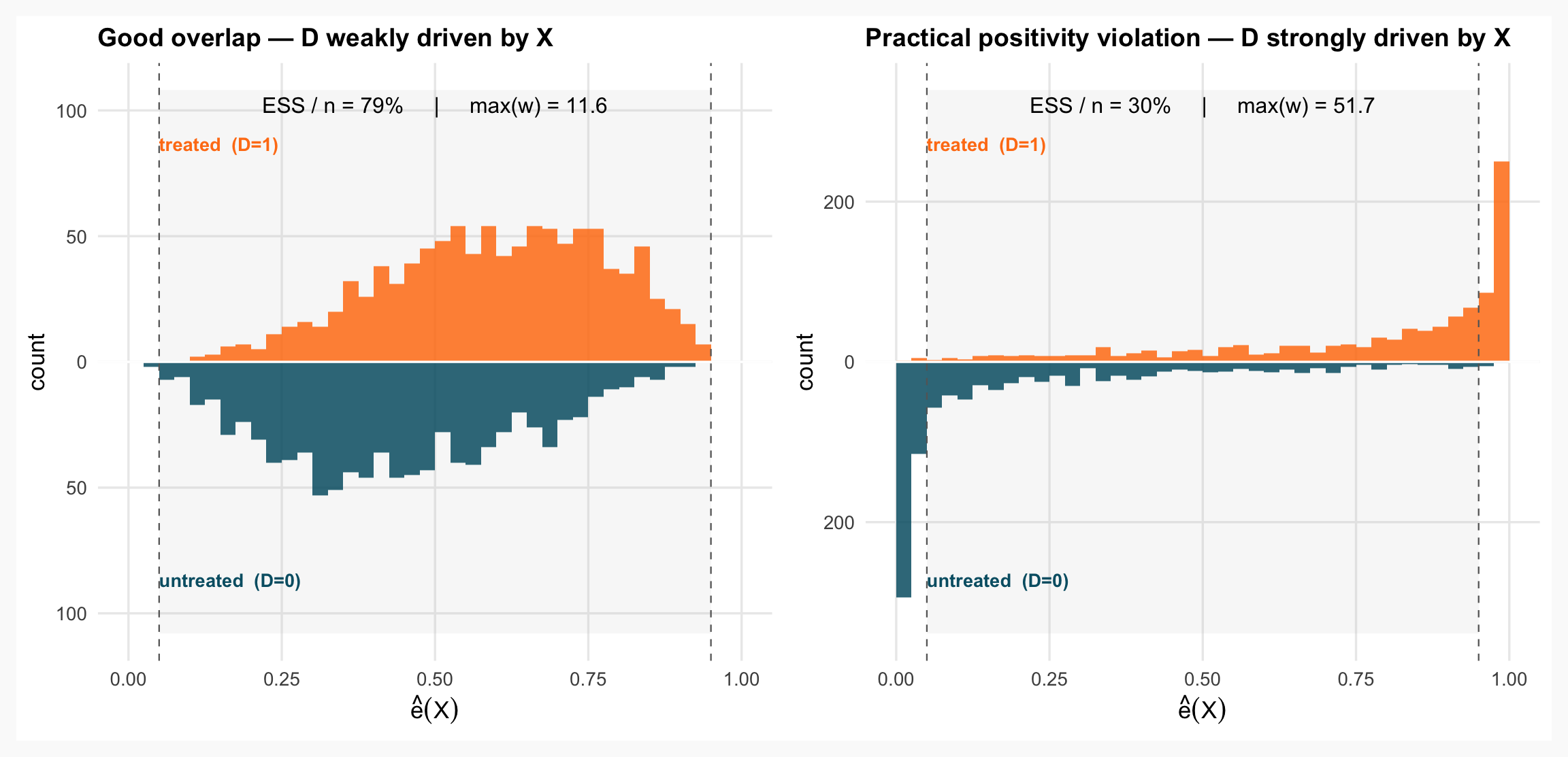
Three diagnostics in one picture. Each unit’s inverse-probability weight is \(w_i = 1/\hat e(\mathbf{x}_i)\) for treated, \(1/(1-\hat e(\mathbf{x}_i))\) for controls. (i) The mirrored histogram of \(\hat e(\mathbf{X})\) — treated above, untreated below — shows where common support holds and where it does not. (ii) ESS / n — the effective sample size \(\text{ESS} = (\sum w_i)^2 / \sum w_i^2\) (Kish), reported relative to \(n\) — collapses when a few units dominate the weights. (iii) max(\(w\)) flags the single most-influential unit. Dashed lines mark the Crump et al. (2009) trim region \([0.05, 0.95]\).

This is the operational picture students need to carry into Ex 3. The mirrored histogram makes positivity visual — both groups should have non-trivial mass across most of \([0,1]\). The ESS-and-max-weight annotations make the practical consequence quantitative: when overlap is bad, a handful of units dominate the estimator. Both panels share the same DGP family — \(D \sim \text{Bernoulli}(\sigma(\beta X))\), \(X \sim N(0,1)\) — varying only \(\beta\). At \(\beta = 1\) the logistic curve is gentle and propensities are spread across \([0.1, 0.9]\); at \(\beta = 3.5\) the curve is steep, propensities concentrate near 0 or 1, and the IPW estimator becomes unstable. Stack 3’s “modern alternatives” slide (entropy balancing, CBPS, SBW, overlap weights) is the remedy menu — Ex 3 asks students to apply two of them on the Stack-2 DGP.

The identification theorem — three equivalent expressions for the ATE

Under Assumption 1 (conditional independence) and Assumption 2 (positivity), the ATE is identified from observed data — in three equivalent ways:

Expression	Formula	Estimator strategy
Adjustment formula	\(\tau = \mathbb{E}_{\mathbf{X}}\!\left[\mathbb{E}(Y \mid D=1, \mathbf{X}) - \mathbb{E}(Y \mid D=0, \mathbf{X})\right]\)	Conditional outcome regression (OR) \(\Rightarrow\) matching or model the OR directly.
IPW	\(\tau = \mathbb{E}\!\left[\dfrac{D \, Y}{e(\mathbf{X})} - \dfrac{(1-D) Y}{1 - e(\mathbf{X})}\right]\)	Model the propensity \(e(\mathbf{X})\) \(\Rightarrow\) inverse-probability weighting.
AIPW	Combine the two with a residual correction (Stack 4).	Model both \(\Rightarrow\) doubly robust.

Three roads to the same ATE. Each row is a separate estimation strategy that motivates one of the next three stacks (Matching → IPW → AIPW).

In population, all three expressions equal \(\tau\). In finite samples, they differ — and the difference comes from which model is misspecified. AIPW’s appeal: it’s consistent if either the OR model or the propensity model is right.

This is the load-bearing identification slide of S06. Memorize the row structure: three equivalent population-level expressions, three different estimator strategies in finite samples. The adjustment formula is the conditional outcome regression form (this is what adjusted OLS is doing implicitly when you regress \(Y \sim D + X\) — though linear OLS is one parametric choice among many). IPW reweights the sample so \(D\) becomes independent of \(X\). AIPW combines both with a correction that makes the estimator robust to misspecification in one of the two models. The pedagogical bridge: every slide in Stacks 2–4 is implementing one of these three rows. The double-robustness intuition (last fragment) is the punchline that motivates Stack 4.

Why adjusted OLS alone is fragile under observational \(D\)

Recall S04: \(Y = \beta_0 + \beta_1 D + \boldsymbol\gamma^\top \mathbf{X} + \varepsilon\), fit by OLS, returns \(\hat\beta_1\) as the ATE under randomization. Under observational \(D\), three things break:

1. Functional-form leak. \(\mathbb{E}(Y \mid D, X)\) is rarely linear-additive. If \(X\) enters non-linearly or interacts with \(D\) (heterogeneous effects), \(\hat\beta_1\) recovers a confounded variance-weighted average, not the ATE (Angrist and Pischke 2009).
2. Extrapolation outside overlap. OLS projects \(\hat\beta_1\) onto the full support of \(X\) even when no treated unit exists at some \(X\). The estimate becomes a model-based extrapolation.
3. Sensitivity to specification. Adding/removing one quadratic term can shift \(\hat\beta_1\) by 30%+ on real data. The “robustness checks” appendix of every empirical paper.

Stack 2 onwards: treat \(\mathbb{E}(Y \mid D, X)\) as a non-parametric object — match on \(X\), weight by \(e(X)\), or combine both — rather than imposing a single parametric form.

OLS does not disappear: in S04 it is the design-justified estimator under random assignment; in S06 it is the baseline and a building block (inside the OR component of AIPW). What changes is the burden of proof.

This is the bridge slide from “Identification” to “Estimation”. Three concrete failure modes — functional-form leak, extrapolation, and specification sensitivity. Each maps to a fix in the next stacks: matching (non-parametric local-linear), IPW (no outcome model at all), AIPW (specification doesn’t need to be right). Students should not leave thinking OLS is “wrong” — it’s a building block. In S04, randomization carried the identification weight and OLS was the optimal estimator. In S06, the analyst’s adjustment set + DAG carry the identification weight; OLS is one (parametric) choice for the OR component. Optional comment: this slide is also the seed for Stack 5’s sensitivity analysis — point #3 says “specification sensitivity”; Cinelli–Hazlett 2020 formalizes “and the sensitivity to unobserved covariates can be benchmarked against the sensitivity to observed ones”.

Conditioning on \(X\), animated — what adjustment actually does

Visual capstone of the Identification section — the adjustment formula in motion. The pooled scatter shows a clear positive treatment–outcome association, but the points split into two clouds by the binary covariate \(X\). Stepping through the animation (highlight groups → compare within group → recombine) shows the pooled slope is largely a between-group artefact; the within-\(X\) (conditional) comparison is the de-confounded effect. This is exactly what “control for \(X\)” means geometrically, and it motivates the rest of S06: how to condition (matching, weighting, AIPW) once \(X\) is high-dimensional. Animation generated natively in R (make_controlforX_gif.R): \(X\) confounds \(D\) and \(Y\) with a true D-effect of 0; the pooled slope of 0.74 collapses to \(\approx 0\) once \(X\) is held fixed. Walk it as raw tilt → colour by \(X\) → within-stratum slopes → partial \(X\) out.

Matching

Build a synthetic RCT by pairing each treated unit with its nearest counterfactual twin.

Open the Matching stack by reframing the identification problem as a sample-construction problem. The adjustment formula expression \(\tau = \mathbb{E}_X[\mathbb{E}(Y|D=1,X) - \mathbb{E}(Y|D=0,X)]\) says: at every value of \(X\), compute the within-X treated-minus-untreated difference, then average across the distribution of \(X\). Matching is the most literal implementation: for each treated unit at \(X_i\), find its untreated twin and take the difference. The whole stack is then a tour of “how to define twin” — exact, Mahalanobis, CEM, propensity-score-based — plus diagnostics and the modern verdict on which method wins. The crucial pedagogical moment is slide 18 (PSM and its discontents): students arrive believing PSM is the standard method (because it’s in every intro textbook); the modern verdict (King-Nielsen 2019) flips that.

Matching idea — pair each treated unit with a comparable untreated unit

The adjustment formula, ATT version: \(\tau_{\text{ATT}} = \mathbb{E}\!\left[\mathbb{E}(Y \mid D=1, X) - \mathbb{E}(Y \mid D=0, X) \mid D=1\right]\).

Matching estimator (1:1, no replacement):

\[\hat\tau_{\text{ATT}} = \frac{1}{n_1}\sum_{i: D_i=1} \bigl(Y_i - Y_{m(i)}\bigr)\]

where \(m(i)\) is the index of unit \(i\)’s “nearest” untreated twin under some distance metric.

Three design choices define a matching algorithm:

1. Distance — exact / Mahalanobis / propensity-based / CEM-coarsened
2. Matching ratio — 1:1 / 1:M / variable-M with caliper
3. Replacement — match-with-replacement reduces bias but inflates variance

For ATE rather than ATT, also match each untreated unit to its treated twin and average: \(\hat\tau_{\text{ATE}} = (n_1/n)\hat\tau_{\text{ATT}} + (n_0/n)\hat\tau_{\text{ATU}}\).

Matching’s appeal is interpretability: every matched pair is a transparent “apples to apples” comparison. The estimator formula is mechanical — pair up, subtract, average. The design choices on this slide are the structural decisions; every estimator on the next slides is a particular cell in the design-choice grid.

ATT vs ATE — why matching natively targets the ATT, and what it costs to push it to the ATE. Matching is built around the treated units’ covariate distribution (we know who got treated), so it estimates the ATT by construction. Going to the ATE means also matching each control to a treated twin to impute the controls’ \(Y(1)\) — and that second direction introduces concerns the ATT avoids:

• Bias (the main one — from overlap). The ATT only needs a comparable control for every treated unit: one-sided support, \(e(X)<1\) on the treated region. The ATE needs \(0<e(X)<1\) everywhere. In observational data the control pool sprawls into regions where treatment essentially never happens (\(e\approx 0\)), so the nearest “treated twin” for those controls is far away → a poor counterfactual → bias. (The Abadie–Imbens matching-discrepancy bias, \(O(N^{-1/k})\) in \(k\) continuous covariates, also accumulates in both directions and is largest exactly where the control→treated matches are worst.)
• Variance. The treated arm is usually the smaller one, so imputing \(Y(1)\) for all controls reuses those few treated units repeatedly (with-replacement / 1:M) → the ATU component is high-variance and the ATE inherits it through the \((n_0/n)\hat\tau_{\text{ATU}}\) term. Matching with replacement is itself the bias↓/variance↑ trade, and it bites harder for the ATE because the small arm must cover the large one.
• Estimand. If overlap is poor, the honest options are to force the off-support matches (bias) or trim to common support — but then you’re estimating the overlap ATE (Crump et al. 2009), not the population ATE. The ATT can stay well-identified when the ATE is not.

It isn’t matching’s fault per se — any ATE estimator needs two-sided overlap (IPW’s \(1/\hat e\) and \(1/(1-\hat e)\) both blow up in the tails) — but matching makes it worse, because its imputation is a hard nearest-neighbour pick rather than a smoothly down-weighted (or overlap-weighted) contribution. So under the usual asymmetric observational overlap, weighting/AIPW with trimming or overlap weights is the gentler ATE tool (Stacks 3–4). And the ATT is often the more meaningful target anyway: “effect on those actually treated” vs. “effect if we treated even units that would never be treated.” The Lalonde lab in Ex 1 produces ATTs — the $1,794 experimental benchmark is itself the ATT — for exactly this reason: matching the NSW treated to PSID controls is credible for the ATT but not for the ATE, where the PSID controls have no comparable treated units.

Matching, animated — pair each treated unit with its nearest control on \(X\)

The matching idea in motion. Start with raw data — a few treated units (teal) among many controls (navy), spread over the covariate \(X\). For each treated unit we scan a caliper window on \(X\) and pair it with its nearest control, then draw the segment. One treated unit sits where there are no comparable controls (the gap near \(X \approx 0.7\)): the caliper drops it, because there is no honest counterfactual on that part of the support — a positivity/overlap failure in miniature, foreshadowing Assumption 2. Averaging the within-pair \(Y\) differences over the matched units recovers the effect (matched ATT ≈ 0.58 vs a true effect of 0.6). This is the visual intuition behind every estimator in the stack: build a synthetic RCT by comparing like with like on \(X\). Animation generated natively in R (make_matching_gif.R).

Exact matching — the conceptual ideal, the curse of dimensionality

Exact matching pairs unit \(i\) with unit \(j\) only if \(\mathbf{X}_i = \mathbf{X}_j\) — coordinate-wise identical.

Why we’d love it: zero bias from the matching step itself. The only assumption needed is overlap.

Why we can’t use it in practice — the curse of dimensionality: with \(K\) binary covariates, \(2^K\) strata; with continuous covariates, the probability of an exact match is zero.

Concrete: 10 binary covariates → 1024 strata. Exact-matching all covariates in a medium-sized data set would leave nearly every treated unit without a twin; even the lab’s example exact match on just four binary covariates strands the continuous ones badly unbalanced.

Two responses:

• Approximate the match (Mahalanobis, propensity, CEM-coarsened) — accept some bias for sample coverage.
• Reduce to a scalar (propensity score, Stack 3) — match in 1-D rather than \(K\)-D.

Exact matching is the pedagogically clean starting point and the operational dead end. The curse of dimensionality kills it on any realistic covariate vector, but it’s worth showing the formal definition because every other matching method is “exact matching with the equality relaxed”. Two responses both surface in the rest of the stack — approximate the match (next 4 slides), or reduce \(X\) to a scalar via the propensity score (slides 17-20).

Mahalanobis distance — covariance-scaled Euclidean

Mahalanobis distance between two covariate vectors:

\[d_M(\mathbf{X}_i, \mathbf{X}_j) = \sqrt{(\mathbf{X}_i - \mathbf{X}_j)^\top \hat\Sigma_X^{-1} (\mathbf{X}_i - \mathbf{X}_j)}\]

where \(\hat\Sigma_X\) is the sample covariance matrix of \(\mathbf{X}\).

Three properties:

• Scale-invariant — multiplying any covariate by 100 doesn’t change the distance.
• Decorrelates — distance treats correlated covariates as a single dimension.
• Continuous — works on continuous and ordinal \(\mathbf{X}\); ill-suited to categorical.

Bias-variance: Mahalanobis preserves more units than exact (lower variance) but accepts non-zero within-pair distance (some bias). Abadie and Imbens (2006) show that, after Mahalanobis matching, a regression bias-correction on the matched pairs — regressing out the residual within-pair covariate gap — further reduces bias.

Mahalanobis matching is the workhorse non-propensity-based matcher. Its appeal is exactness-of-the-metric (no model fit) combined with practical sample coverage. Two pedagogical points: scale invariance and decorrelation. Abadie–Imbens (2006) additionally bias-correct the matched pairs by regressing out the residual within-pair covariate gap with an arm-specific outcome model (Matching::Match(BiasAdjust = TRUE); MatchIt does the matching only — the correction is the outcome regression you fit afterwards). This reduces bias, which is a separate question from SE validity — see the inference slide (valid SEs need the Abadie–Imbens analytic variance or matched-set cluster-robust SEs, not plain robust SEs). Mention briefly that pure Mahalanobis breaks down with many categorical covariates (rank-deficient \(\hat\Sigma_X\)); the practical workaround is “Mahalanobis on continuous + exact on categorical”, which MatchIt supports via exact = c(...).

Coarsened Exact Matching (CEM) — bin, then match exactly within bins

Iacus, King, and Porro (2012): bin each continuous covariate into a small number of strata, then do exact matching on the bins. Treated units in bins with no untreated unit (or vice versa) are pruned from the sample.

Example: age in years → age in 5-year bins {18–22, 23–27, …}; income → quintile.

The MIB property (Monotonic Imbalance Bounding): the user sets the maximum within-bin imbalance — formally the L1 distance between the treated and control covariate histograms, CEM’s native metric — via the coarsening width, so bias is bounded before the data are touched. Other methods (PSM, Mahalanobis) only let the analyst diagnose imbalance ex post.

The price is sample loss: aggressive coarsening preserves balance at the cost of pruning units; the estimand effectively becomes the ATT on the overlap region.

Software: MatchIt::matchit(method = "cem") in R (wraps the cem package); no canonical Python implementation — coarsen each covariate by hand (pandas.cut / qcut) and exact-match within bins, or call R from Python via rpy2.

CEM is the modern recommendation for matching when sample size permits the pruning. The MIB property is the headline pedagogical point — it inverts the usual workflow. With PSM/Mahalanobis, you match first and then check balance with cobalt; if balance is bad, you re-specify the model and try again, garden-of-forking-paths. With CEM, you fix the maximum allowed imbalance up front via the coarsening; the algorithm prunes the units that don’t fit. Bias is bounded by construction. The price is sample loss and the implicit redefinition of the estimand to “ATT on the CEM-pruned subsample” — this is fine if you report it transparently. The Ex 1 lab shows the flip side: CEM’s MIB property bounds within-bin imbalance only on the coarsening grid, and default coarsening on Lalonde prunes so aggressively (51 of 185 treated retained) that the retained sample is badly balanced (max |SMD| ≈ 0.63) and the ATT lands far off (≈ −$3,013). Mahalanobis is the method that converges.

CEM, animated — coarsen \(X\) into bins; a bounded gap survives inside each

The MIB property in motion, as a coarsening dial. Each continuous covariate \(X\) is binned, and treated units are matched exactly on the bins. Narrow bins (\(w = 0.05\)): the residual within-bin gap — the leftover treated-minus-control difference in the un-coarsened \(X\) — is tiny, so balance is tight, but many units land in single-group bins and are pruned (greyed, orange ✕, the same drop idiom as matching.gif). Turn the dial wider and the trade reverses: fewer units pruned, but every orange gap whisker lengthens. The key reading: exact-matching on the bins is not exact-matching on \(X\) — a residual gap survives inside every retained bin, and it can never exceed the bin width \(w\). That is exactly the MIB property from the previous slide: you set the maximum within-bin imbalance up front by choosing \(w\), before touching the outcome (note there is no \(Y\) axis here — CEM is a pre-outcome design step). The orange gap echoes the orange ATT accent from matching.gif: same colour, “the quantity we care about”. The price is sample loss (the pruned units) and an estimand quietly redefined to the ATT on the retained overlap. The Ex 1 Lalonde lab is the cautionary version: default coarsening prunes so hard (51 of 185 treated retained) that the retained sample is badly balanced (max |SMD| ≈ 0.63) and the ATT lands far off (≈ −$3,013) — MIB bounds the coarsening grid, not the retained sample’s representativeness. Animation generated natively in R (make_cem_coarsening_dial.R), sibling to matching.gif.

1:M, replacement, caliper — the bias-variance dial

Three more design knobs, all on a bias–variance tradeoff:

Design choice	Bias effect	Variance effect	Default
1:M (M>1) matching	Higher (more imperfect matches per treated unit)	Lower (more data in each \(\hat\mu_0\))	\(M \in \{2, 4\}\)
With replacement	Lower (each treated gets its actual nearest neighbour)	Higher (some controls appear in many pairs)	Yes
Caliper \(c\)	Lower (drops matches with \(d > c\))	Higher (smaller matched sample)	\(c = 0.2 \cdot \sigma_{\text{logit}(e)}\)

Caliper rule of thumb (Rosenbaum and Rubin 1985): caliper = 0.2 × the standard deviation of the logit of the propensity score. Drops units with no acceptable twin within that range.

Modern practice: match with replacement + 1:M (\(M=4\)) + caliper 0.2; report the number of unique controls used and the share of treated units that found a match within the caliper.

This slide is the “knobs you can turn” reference. Default settings on the right column are the consensus-in-applied-econ defaults. The caliper rule of thumb (0.2 × SD of the logit PS) is Rosenbaum & Rubin 1985, still the standard. Match-with-replacement is the modern default because it reduces bias more than it inflates variance in any sample where unmatched controls would otherwise be discarded. Modern practice (last fragment) is the “what should I do” actionable summary: 1:4 with replacement + caliper 0.2 is the default in MatchIt and is what psmpy mimics. Report transparency requires the share-of-treated-matched number — if 30% of treated are dropped because no match exists within the caliper, the ATT you’re estimating is no longer on the original treated population, it’s on the matchable subset.

Balance diagnostics — the standardized mean difference and the Love plot

Standardized mean difference for covariate \(X_k\) after matching:

\[\text{SMD}_k = \frac{\bar X_{k,1} - \bar X_{k,0}}{\sqrt{(s_{k,1}^2 + s_{k,0}^2)/2}}\]

Rule of thumb: \(|\text{SMD}_k| < 0.10\) = balance achieved (Stuart 2010).

The Love plot shows each covariate’s absolute SMD before vs. after matching — cobalt::love.plot(): one row per covariate, dashed line at 0.10. Richer checks — variance ratio, K-S — come next.

The operational diagnostic slide. SMD < 0.10 is the consensus rule (Stuart 2010, Statistical Science). The Love plot — named after Thomas E. Love — is cobalt’s one-liner: each covariate is a row, its absolute SMD shown before (orange) and after (navy) matching, with a dashed threshold at 0.10. On this simulated 1:1 NN-PSM sample, income is pulled from ~0.89 down to ~0.22 but stays above the line, age lands on it, the rest clear it. Reporting standard: a Love plot plus a numerical SMD table, before and after. Anything still above 0.10 — here income, marginally age — is regressed out by adding those covariates to a final outcome model on the matched sample (the same residual-gap logic as the Abadie–Imbens 2006 bias correction, though not literally that matching-imputation estimator), rather than re-matching endlessly; pair it with matched-set cluster-robust SEs, not plain HC1. The same plot with a different statistic gives the variance-ratio and K-S checks on the next slide. (Figure: make_loveplot.R.)

Beyond the mean — variance ratio and K-S

SMD compares means only. The same Love plot, with a different statistic, checks more:

• Variance ratio \(s_{k,1}^2 / s_{k,0}^2 \in [0.5, 2]\) — the second moment (spread); means can match while variances don’t.
• K-S statistic — the largest gap between the two covariates’ CDFs — the whole marginal distribution (shape, skew, multimodality).

love.plot(stats = c("variance.ratios", "ks.statistics")). Here spread is fine everywhere (ratios near 1), but income is flagged on K-S too — its whole distribution is shifted, not just its mean. Today’s lab stays on SMD.

SMD only checks the first moment. The variance ratio catches the second — a covariate whose mean matches but whose spread doesn’t (ratio outside [0.5, 2]); here all variance ratios sit near 1, so spread was never the problem in this sample. The K-S statistic compares the entire marginal CDF, catching shape differences both means and variances miss — income is flagged on K-S as well as SMD (previous slide), confirming its whole distribution is shifted, not just its mean. Both are per-covariate, so love.plot() draws them as panels via stats=, in the same row order as the SMD plot so you can read across. The Ex 1 lab stays on SMD — these are enrichment, not required there. (The multivariate L1 imbalance — the whole-joint-distribution analogue — lives with CEM, whose MIB property bounds it by construction.)

Propensity score — Rosenbaum–Rubin’s dimensionality reduction trick

Propensity score = \(e(\mathbf{X}) = P(D = 1 \mid \mathbf{X})\) — the conditional probability of treatment.

Rosenbaum–Rubin (1983) balancing-score theorem:

Theorem

If \((Y(0), Y(1)) \perp D \mid \mathbf{X}\), then \((Y(0), Y(1)) \perp D \mid e(\mathbf{X})\).

Translation: conditioning on the scalar \(e(\mathbf{X})\) achieves the same balance as conditioning on the full vector \(\mathbf{X}\) (Rosenbaum and Rubin 1983).

\(e(\mathbf{X})\) is a sufficient statistic for \(\mathbf{X}\) as a confounder: it absorbs every backdoor that \(\mathbf{X}\) does.

Why it matters operationally: match in 1-D instead of \(K\)-D. Curse of dimensionality, dodged.

The Rosenbaum-Rubin theorem is the theoretical foundation of every propensity-based method. The key word is “balancing score” — \(e(\mathbf{X})\) is the coarsest function of \(\mathbf{X}\) that still satisfies the balancing property. Students who internalize this slide can read every PSM paper without confusion. The DAG on the right shows \(\mathbf{X}\) entering the confounding path through \(e\); conditioning on \(e\) blocks the backdoor just as conditioning on \(\mathbf{X}\) would. The 1-D reduction is the practical motivation. Next slide will show how to estimate \(e\) and use it to match.

Propensity score matching — match on \(\hat e\), not on \(\mathbf{X}\)

Three steps:

1. Estimate the propensity score. Fit a binary-choice model: \(\hat e(\mathbf{x}) = \Lambda(\hat\beta_0 + \hat{\boldsymbol\beta}^\top \mathbf{x})\) where \(\Lambda\) is logit (or probit, or — modern — gradient-boosted trees / a neural net).
2. Match on \(\hat e\). Each treated unit’s twin is the untreated unit with the closest \(\hat e\) (1:1) or the \(M\) closest (1:M, optionally with caliper).
3. Estimate \(\hat\tau_{\text{ATT}}\) by averaging the paired differences. For the SE, use the Abadie–Imbens (2006) analytic variance, or matched-set cluster-robust SEs on the matched-sample regression — not plain HC1 or the naïve bootstrap (see the inference slide).

This was the dominant matching method from 1983 (Rosenbaum–Rubin) to ~2019. Then King & Nielsen published a paper that changed the consensus.

PSM is the textbook matching method and was the operational default for 35 years. Pedagogically, this slide presents it neutrally (as students will read in any pre-2020 textbook) before the next slide pivots to the modern critique. The “modern” alternatives in step 1 — gradient-boosted trees, neural nets — are increasingly common; this is where the propensity score gets ML treatment. But there’s a subtle issue: ML propensity scores can produce extreme weights and overfit; we’ll return to this in S08 (DML’s cross-fitting solves the overfit problem).

PSM and its discontents — King & Nielsen 2019

“Why Propensity Scores Should Not Be Used for Matching” (Political Analysis, 2019)

King and Nielsen (2019) show, both theoretically and via simulation, that propensity score matching can increase imbalance relative to no matching, because matching on \(\hat e\) approximates random sampling within strata of \(\hat e\) — which has nothing to do with covariate-level balance.

Three takeaways for practitioners:

1. PSM imitates a completely randomized experiment, not a fully blocked one. In a complete-RCT, covariates are balanced in expectation, not in every sample.
2. CEM and Mahalanobis imitate a fully blocked experiment — covariate balance is enforced sample by sample.
3. The “propensity score paradox”: the better your PSM model fits, the more it converges to random matching within strata, and the worse your covariate balance can get.

Operational rule: prefer covariate-space matching (CEM or Mahalanobis) over PSM for matching — but choose between them by checking both balance and retained-sample representativeness: CEM can over-prune (as in today’s Lalonde lab), in which case Mahalanobis is the better choice. Reserve the propensity score for weighting (Stack 3) and AIPW (Stack 4), where its mathematical role is different.

This is the pivotal slide of Stack 2. Students will have read about PSM in every introductory causal-inference textbook; this slide is the update. The simulation in King-Nielsen 2019 is the empirical pillar: they show that for any reasonable PSM specification, varying the random-matching step’s seed produces ATT estimates with sufficient variance to include and exclude zero — i.e., the “matching” step is partially randomized noise. The deeper theoretical point (the “PSM paradox”) is the subtle part: a well-specified PSM model produces concentrated propensities, which means within-stratum matching becomes random sampling, which destroys the within-stratum covariate balance. CEM and Mahalanobis avoid this because they match on the actual covariates, not on a 1-D summary. The operational takeaway is the actionable bit: prefer covariate-space matching (CEM or Mahalanobis) over PSM, choosing between them by balance and retained-sample size — in today’s Lalonde lab CEM over-prunes and Mahalanobis wins. The propensity score still has its role, but it’s IPW/AIPW, not matching. The Ex 1 lab will reproduce this in miniature on Lalonde.

Estimation after matching — what works, what doesn’t

The point estimate is easy — the (weighted) average paired difference. The standard error is the subtle part: the matched sample is constructed, not an i.i.d. draw.

Does not work:

• ❌ Naïve t-test — matched pairs aren’t i.i.d.; they share controls.
• ❌ Naïve bootstrap of the matching procedure — not consistent for matching SEs (Abadie and Imbens 2008).
• ❌ Plain HC1 on the matched sample — treats it as i.i.d.; inconsistent, and errs in either direction (Abadie and Spiess 2022).

Works — two valid routes:

• ✅ Abadie–Imbens analytic SEs — a matching-aware variance.
• ✅ Matched-sample regression + matched-set cluster-robust SEs.

How the two relate, and how to run them — next.

The point estimate is mechanical; the SE is subtle because the matched sample is built by the analyst (units selected, controls possibly reused), so it is not an i.i.d. sample. Three failure modes are common in student work: the naive paired t-test (ignores the shared-control dependence), the naive nonparametric bootstrap (Abadie–Imbens 2008 published a counterexample — it can be anti-conservative), and plain HC1 on the matched sample (Abadie–Spiess 2022: inconsistent, and the error flips sign across DGPs, so not even reliably conservative). Two routes are valid; they are unpacked on the next slide. Keep this slide at the level of “what works / what doesn’t” — the how is next.

Two valid routes to the SE — same estimand, complementary checks

Same estimand, same probability limit → two complete (estimator + SE) packages. Pick one to report; run both as a robustness check. Don’t mix the parts — or fall back to HC1.

A · Abadie–Imbens (matching-aware)

Matching-imputation + a regression bias-correction — subtract the predicted gap \(\hat\mu(\mathbf{X}_i) - \hat\mu(\mathbf{X}_{m(i)})\) (gap × slope) + the AI analytic variance.

library(Matching)
m <- Match(Y, Tr = D, X,    # X = covars / PS
           estimand = "ATT",
           Weight = 2,      # 2 = Mahalanobis
           replace = TRUE,
           BiasAdjust = TRUE)
m$est   # ATT
m$se    # AI analytic variance

B · Matched-sample regression

Weighted \(Y \sim D + \mathbf{X}\) on the matched data — adding \(\mathbf{X}\) regresses out residual imbalance — + matched-set cluster-robust SEs.

m  <- matchit(D ~ X1 + X2 + ..., method = "cem")
md <- match.data(m)         # weights, subclass
lm_robust(Y ~ D + X1 + X2 + ...,
          data = md, weights = weights,
          clusters = subclass,  # +id if replace
          se_type = "CR2")      # not HC1

Caveat: CEM isn’t in the Matching package, so route A covers exact / Mahalanobis / PSM.

The two routes are complementary, not either/or. They target the same estimand (ATT/ATE under unconfoundedness) and share a probability limit, so each is a complete (estimator + variance) package and a careful analyst reports both as a robustness check. Route A (Abadie–Imbens, the Matching package) is matching-imputation with the regression bias correction (the gap × slope term) and the AI analytic variance — valid for matching with replacement. Route B (matched-sample regression) fits a weighted \(Y \sim D + X\) and pairs it with matched-set cluster-robust SEs: cluster by subclass without replacement, by subclass and the reused-unit id (via get_matches()) with replacement. The variances are NOT interchangeable across routes — each is derived for its own estimator — and neither is plain HC1. On the Ex 1 Lalonde data the routes agree on the qualitative story but differ in the exact numbers (route B Mahalanobis ATT ≈ 1,941, cluster-SE ≈ 1,162; route A bias-corrected ≈ 2,520, AI SE ≈ 1,705), with the AI SE more conservative; Matching::Match defaults to averaging tied matches (ties = TRUE) where MatchIt picks one, which is part of the gap. CEM is not in the Matching package, so route A can’t do all six methods. The code blocks are illustrative (r, not executed) so the deck takes no Matching-package dependency at render.

Inverse Probability Weighting

Weight every observation by 1 / its probability of being where it is — and the sample becomes as-if-randomized.

Concretely: where treatment is rare (\(\hat e = 0.2\)), up-weight each treated unit by \(1/0.2 = 5\) so it stands in for the four like it — rebuilding the pseudo-population.

Stack 3 opens with the second of the three identification expressions: IPW. The “concretely” subtitle is the pseudo-population intuition behind the \(1/\hat e\) weight — surfaced here at the section opener so the theorem slide can stay formula-clean. The pedagogical bridge from matching: matching removes observations (controls without a treated twin); IPW reweights every observation, keeping the full sample. The 1/PS weight is the up-weighting that compensates for the treated unit’s under-representation in regions of \(\mathbf{X}\) where treatment was unlikely. Stack outline: theorem (Horvitz-Thompson), Hájek normalization, diagnostics, modern balancing weights, worked DGP example (Ex 2), inference.

IPW theorem — Horvitz–Thompson reweighting recovers the ATE

Theorem (Horvitz–Thompson)

Under conditional independence (\(Y(0), Y(1) \perp D \mid \mathbf{X}\)) and positivity (\(0 < e(\mathbf{X}) < 1\)):

\[\tau_{\text{ATE}} = \mathbb{E}\!\left[\frac{D \, Y}{e(\mathbf{X})} - \frac{(1-D) \, Y}{1 - e(\mathbf{X})}\right]\]

Proof sketch (for the \(\mathbb{E}[Y(1)]\) piece):

\[\mathbb{E}\!\left[\frac{D \, Y}{e(\mathbf{X})}\right] = \mathbb{E}\!\left[\mathbb{E}\!\left(\frac{D \, Y(1)}{e(\mathbf{X})} \,\bigg|\, \mathbf{X}\right)\right] = \mathbb{E}\!\left[\frac{\mathbb{E}(D \mid \mathbf{X}) \, \mathbb{E}(Y(1) \mid \mathbf{X})}{e(\mathbf{X})}\right] = \mathbb{E}[\mathbb{E}(Y(1) \mid \mathbf{X})] = \mathbb{E}[Y(1)]\]

Sample estimator: plug in \(\hat e(\mathbf{X}_i)\):

\[\hat\tau_{\text{ATE}}^{\text{HT}} = \frac{1}{n}\sum_{i=1}^n \frac{D_i Y_i}{\hat e(\mathbf{X}_i)} - \frac{1}{n}\sum_{i=1}^n \frac{(1-D_i) Y_i}{1 - \hat e(\mathbf{X}_i)}\]

The IPW theorem is one of the cleanest results in observational causal inference. The proof uses only iterated expectations and the conditional independence assumption — no parametric model, no functional-form assumption on \(Y\). The Horvitz–Thompson form is the original 1952 sampling formulation (HT 1952 was a survey-sampling paper); Hirano-Imbens-Ridder 2003 proved its asymptotic efficiency in the causal-inference context. The sample-version formula in the third fragment is what we’ll compute in the Ex 2 lab. Pedagogically, the trick is to notice that this is “S04’s outcome-side equation, but instead of the experimenter making \(\mathbb{E}[D|X]\) equal to a known constant, we estimate it and divide by it”.

Hájek (normalized) IPW — same idea, smaller variance

The Horvitz–Thompson estimator divides by \(n\). The Hájek version divides by the sum of weights:

\[\hat\tau_{\text{ATE}}^{\text{Hájek}} = \frac{\sum_i D_i Y_i / \hat e_i}{\sum_i D_i / \hat e_i} - \frac{\sum_i (1-D_i) Y_i / (1-\hat e_i)}{\sum_i (1-D_i) / (1-\hat e_i)}\]

Why Hájek is preferred in practice:

• Lower variance when weights are skewed (almost always): HT divides by a fixed \(n\), so one giant \(1/\hat e_i\) inflates the mean; Hájek self-normalizes — dividing by the realized \(\sum_i D_i/\hat e_i\) — so numerator and denominator inflate together and partly cancel.
• Each arm-mean is a weighted average of observed \(Y\) — so each lies in \([\min Y, \max Y]\) (the flip side of that cancellation); the HT arm-means do not.
• Invariant to shifting \(Y\) by a constant.

Bias-variance: HT is unbiased but high-variance; Hájek’s tiny \(O(1/n)\) bias — negligible beside its own \(O(1/\sqrt n)\) SE — buys much lower variance and lower MSE. The practical default.

The Hájek version is what every software package actually implements when you ask for “IPW” — WeightIt, survey, IPW. The HT form is the textbook starting point but is almost never used in practice because its variance blows up when even one weight is large. The third fragment is the technical caveat for students who took mathematical-statistics: Hájek is biased in finite samples, HT is unbiased but high-variance. We almost always pick lower-variance-biased-O(1/n) over unbiased-blow-up. Tie this to S05’s earlier theme: bias-variance trades are pervasive; the choice of estimator is choice of where on the curve you sit.

Diagnostics — weight tails, ESS, trimming

When \(\hat e(\mathbf{X}_i) \to 0\) or \(\to 1\) for some \(i\), the inverse weight \(\to \infty\) — a single observation can dominate the estimator.

Three diagnostics:

Diagnostic	Formula	Action threshold
Max / min weight	\(\max_i w_i\) and \(\min_i w_i\)	Investigate any \(w_i > 10\) or \(> 0.1n\).
Effective sample size	\(\text{ESS} = \big(\sum_i w_i\big)^2 / \sum_i w_i^2\) i.i.d.-equivalents: ESS = 0.5n ⇒ 1000 rows carry the info of 500 equally-weighted obs.	ESS \(< 0.5n\) ⇒ heavy concentration.
Propensity histogram	\(\hat e(\mathbf{X}_i)\) by group \(D\)	Near-zero mass for either tail ⇒ trim.

Trimming rule: drop units with \(\hat e \notin [\alpha, 1-\alpha]\), typically \(\alpha = 0.05\) or \(0.1\). The estimand becomes the ATE on the overlap region; report this change transparently (Crump et al. 2009).

Modern alternative — overlap weights: weight by \(e(1-e)\) instead of \(1/e\) or \(1/(1-e)\). No discontinuous trimming; the weight smoothly down-weights extreme propensities (Li, Morgan, and Zaslavsky 2018).

This is the operational “is my IPW broken” diagnostic slide. The ESS formula is the Kish (1965) effective-sample-size — analogous to the design effect in survey sampling. The trimming rule of Crump et al. is the standard, but it’s a discontinuous treatment of \(\hat e\); the overlap-weights alternative (Li-Morgan-Zaslavsky 2018) is increasingly the modern default because it preserves all units and changes the estimand to a quantity that’s both well-defined and clinically interpretable (ATE on the “equipoise” population — those with non-trivial probability of either treatment). Ex 3 will compute all three diagnostics and demonstrate trimming (on a deliberately stressed DGP).

IPW weights, made visual — a heavy tail is a positivity failure

This is the companion to the diagnostics table — the same three diagnostics (max weight, ESS, the trim region), now visual, and built on the exact β = 3.5 DGP from the Stack-1 “Positivity at a glance” slide so students see the mirrored ê(X) histogram and the weights it produces as two views of one phenomenon. The headline lesson: a heavy weight tail is not a nuisance to winsorize away quietly — it is positivity failing, and trimming it changes the estimand to the overlap ATE. Ex 3 reproduces this on the stressed DGP and adds overlap weights + entropy balancing as the no-trimming alternatives.

Modern balancing weights — enforce-by-design

Standard IPW: fit a propensity model \(\hat e(\mathbf{X})\) → invert → check balance ex post — the weighted Love plot / SMD check from Stack 2, now on the weighted sample. If balance is bad, re-specify and try again.

Modern alternative (Athey and Imbens 2017): enforce balance as weight constraints rather than ex-post from a fitted model.

Method	Idea — the constrained weight problem
Entropy balancing (Hainmueller 2012) · ebal, WeightIt	Balance becomes a hard constraint, not a hope: the weights reproduce the treated covariate means exactly. Among all weightings that do, the max-entropy objective (minimize negentropy = minimize KL-from-uniform) picks the one closest to uniform — disturbing the sample as little as balance allows. \(\min_w \sum_i w_i \log w_i \;\;\text{s.t.}\;\; \sum_i w_i \mathbf{X}_i = \bar{\mathbf{X}}_{\text{treat}}\)
Covariate balancing PS (Imai and Ratkovic 2014) · CBPS	Ordinary logistic PS maximizes fit to who got treated — good prediction, but not necessarily good balance. CBPS estimates the same score while adding balance as a moment condition, so one model does double duty: predict treatment and equalize covariate means (solved by GMM). \(\sum_i\!\big(\tfrac{D_i}{\hat e_i}-\tfrac{1-D_i}{1-\hat e_i}\big)\mathbf{X}_i = 0\)
Stable balancing weights (Zubizarreta 2015) · sbw	The mirror image of entropy balancing: instead of exact balance at any cost, you cap the tolerable imbalance \(\delta\) and the solver returns the least-variable weights that stay inside it. Minimizing weight spread keeps the effective sample large — dialing bias (\(\delta\)) against variance directly. \(\min_w \sum_i w_i^2 \;\;\text{s.t.}\;\; \big|\sum_i w_i \mathbf{X}_i - \bar{\mathbf{X}}_{\text{target}}\big| \le \delta\)

This is the modernization slide for Stack 3. Entropy balancing is the most accessible of the three; its objective is to find weights that minimize KL-divergence from uniform subject to “first \(k\) moments of treated and control match exactly”. Zubizarreta’s stable balancing weights flip the constraint: user picks the tolerable imbalance, the solver finds the minimum-variance weights. CBPS is in between: fits the propensity model under a balancing objective rather than maximum likelihood. The Athey-Imbens 2017 JEP article is the canonical citation for “modern applied causal inference recommends these” — it’s free online and assigned in many graduate courses.

Doubly Robust: AIPW

Combine the outcome model and the propensity model — and get two chances to be right.

Stack 4 is the synthesis of Stacks 2 and 3. The adjustment formula (used implicitly by matching and OLS) needs the outcome model to be right; IPW needs the propensity model to be right. AIPW combines them — and the magic is that AIPW is consistent if either is correct, not necessarily both. This is the double robustness property. Origin: Robins-Rotnitzky-Zhao 1994 (JASA); modern presentation: Bang & Robins 2005 (Biometrics). Pedagogically, AIPW is also the building block for S08’s DML (cross-fitted AIPW with ML nuisances), so this stack ends with a forward-pointer.

AIPW idea — augment the OR, or augment the IPW

Ingredients: outcome regression \(\hat\mu_d(\mathbf{x}) = \hat{\mathbb{E}}(Y \mid D{=}d, \mathbf{X}{=}\mathbf{x})\) and propensity score \(\hat e(\mathbf{x}) = \hat P(D{=}1 \mid \mathbf{X}{=}\mathbf{x})\). The same estimator regroups two equivalent ways (Robins, Rotnitzky, and Zhao 1994):

(A) Augment the OR — adjustment formula, corrected by an IPW-weighted residual:

\[\hat\tau_{\text{AIPW}} = \frac{1}{n}\sum_i\Big[\,\underbrace{\hat\mu_1 - \hat\mu_0}_{\text{OR difference}} \;+\; \underbrace{\tfrac{D_i(Y_i-\hat\mu_1)}{\hat e} - \tfrac{(1-D_i)(Y_i-\hat\mu_0)}{1-\hat e}}_{\text{IPW correction on the OR residual}}\,\Big]\]

OR right ⇒ residuals are mean-zero ⇒ a wrong PS does no harm.

(B) Augment the IPW — Horvitz–Thompson, corrected by the outcome model:

\[\hat\tau_{\text{AIPW}} = \frac{1}{n}\sum_i\Big[\,\underbrace{\tfrac{D_i Y_i}{\hat e} - \tfrac{(1-D_i)Y_i}{1-\hat e}}_{\text{IPW (Horvitz–Thompson)}} \;-\; \underbrace{(D_i-\hat e)\big(\tfrac{\hat\mu_1}{\hat e} + \tfrac{\hat\mu_0}{1-\hat e}\big)}_{\text{OR correction}}\,\Big]\]

PS right ⇒ \(D_i-\hat e\) is mean-zero ⇒ a wrong OR does no harm.

The AIPW formula is the central algebraic object of Stack 4. Forms (A) and (B) are the identical sum regrouped — (A) leads with the OR difference and collects the \(\hat\mu\) terms, (B) leads with the Horvitz–Thompson IPW estimator and collects the \(Y\) terms; they are numerically equal for any \(\hat\mu, \hat e\) (verified to machine precision — it’s pure algebra, not an approximation). Reading both is the pedagogical key to double robustness: in (A) the augmentation residual is mean-zero when the OR is right, so a wrong PS washes out; in (B) the correction carries the factor \(D_i-\hat e\), which is mean-zero when the PS is right, so a wrong OR washes out. Either model being right is enough. Caution on the board: the (B) correction is subtracted, and \((D_i-\hat e)\) can be negative — students sometimes flip the sign. The Bang-Robins 2005 paper (Biometrics) is the cleanest modern presentation; RRZ 1994 (JASA) is the original.

Double robust — consistent if either model is right

Theorem (Double Robustness)

Under conditional independence and positivity, \(\hat\tau_{\text{AIPW}} \xrightarrow{p} \tau_{\text{ATE}}\) if either:

• \(\hat\mu_d \xrightarrow{p} \mu_d\) (OR correctly specified), or
• \(\hat e \xrightarrow{p} e\) (PS correctly specified) — or both.

Proof intuition. The bias of AIPW decomposes:

\[\mathbb{E}[\hat\tau_{\text{AIPW}}] - \tau = \mathbb{E}\!\left[\underbrace{\left(\frac{e - \hat e}{\hat e}\right)}_{\text{PS error}} \cdot \underbrace{(\mu_1 - \hat\mu_1)}_{\text{OR error}}\right] + (\text{symmetric for } d=0)\]

The bias is the product of the two errors — small if either factor is small.

Failure mode: if both are wrong, AIPW is biased — “two chances”, not bullet-proof. And both chances live inside conditional independence (same \(\mathbf{X}\)): an omitted confounder breaks both at once. DR guards functional form, not identification → Sensitivity Analysis.

This is the load-bearing theoretical slide of Stack 4. The product-of-errors decomposition (Bang-Robins 2005) is the cleanest way to see why DR works: the bias is the product of the two model errors, so it’s small if one factor is small. This is also why AIPW combined with ML nuisances (S08 DML) is powerful — ML estimators converge slowly individually (often at \(n^{-1/4}\)), but the product of two \(n^{-1/4}\) errors is \(n^{-1/2}\), which is the rate \(\sqrt{n}\)-consistency requires. That’s the Chernozhukov et al. 2018 insight; we’ll formalize it in S08. The failure-mode fragment is the honest caveat: AIPW does not save you from a wholly wrong DAG.

AIPW inference — the influence function gives the SE

AIPW is asymptotically linear: \(\hat\tau \approx \tau + \tfrac{1}{n}\sum_i \psi(O_i)\) with \(\mathbb{E}[\psi]=0\). The influence function \(\psi(O_i)\) is how much one observation moves the estimate; the CLT then gives \(\sqrt n\,(\hat\tau-\tau)\xrightarrow{d} N\!\big(0,\,\mathbb{E}[\psi^2]\big)\).

For AIPW, \(\psi\) is just the centered per-unit contribution from the estimator — its efficient influence function (which is why AIPW attains the efficiency bound (Hirano, Imbens, and Ridder 2003)):

\[\hat\psi_i = \underbrace{\hat\mu_1 - \hat\mu_0 + \tfrac{D_i(Y_i-\hat\mu_1)}{\hat e} - \tfrac{(1-D_i)(Y_i-\hat\mu_0)}{1-\hat e}}_{i\text{-th AIPW contribution}} \;-\; \hat\tau\]

\[\widehat{\operatorname{SE}}(\hat\tau_{\text{AIPW}}) \;=\; \frac{\operatorname{sd}(\hat\psi_i)}{\sqrt n}\]

the spread of the per-unit contributions, over \(\sqrt n\) — no delta method. (Ex 3 bootstraps it; econml.dr.LinearDRLearner returns it analytically.)

This slide reframes AIPW inference around the influence function. Key point: AIPW is asymptotically linear, so its sampling distribution is governed by a single mean-zero function ψ — and for AIPW that ψ is literally the centered per-unit summand from the two-forms slide. So the SE needs no delta method: take each row’s AIPW contribution, centre at τ̂, compute the sample SD, divide by √n (this equals the Var(ψ)/n plug-in the software returns). That ψ is the efficient influence function is exactly why AIPW attains the semiparametric efficiency bound — so old properties 2 (efficiency) and 3 (asymptotic normality) are both statements about ψ; double robustness (old property 1) is now its own slide. DELIBERATE SCOPE: we stop at the IF as an inference device here. The deeper property — that ψ is Neyman-orthogonal, i.e. first-order insensitive to errors in the nuisances (the same product-of-errors fact as the DR theorem), which is what licenses slow ML nuisance estimators — is the conceptual core of S08 (DML) and is introduced there, not here. (The full-sample anti-conservative-CI caveat — reusing rows to fit and evaluate makes IF-CIs too narrow when the nuisances have many covariates (large K, relative to n) — now lives on the Bridge-to-S08 slide, where cross-fitting is the fix.) Practical: Ex 3 bootstraps the SE (its forest-plot reflection question); econml’s LinearDRLearner returns the analytic IF SE.

Double robustness, visualized — the CI covers the truth whenever one model is right

AIPW’s CI covers the truth (teal) wherever one model is right — A, B, and C — missing only D; IPW-alone covers A/B, OR-alone A/C. DR = teal in three panels of four.

This delivers the forest plot specified in Ex 3 Q2 (the four-scenario double-robustness demo — A both right, B OR wrong, C PS wrong, D both wrong). Generated natively (make_aipw_dr_forest.R) on the exact Ex 2 DGP with bootstrap CIs; the coverage pattern is the theorem made empirical — AIPW covers 2.0 in A/B/C, IPW-alone only when its propensity model is right (A/B), OR-alone only when its outcome model is right (A/C), and nothing covers in D. Students reproduce this in the lab. The colour encodes the punchline: count the teal intervals per estimator — AIPW wins 3-of-4, the single-model estimators 2-of-4 each.

Bridge to S08 — AIPW + cross-fitting + ML nuisances = DML

AIPW with logistic PS and linear OR is the classical setup — but on the full sample, fitting and evaluating the nuisances on the same rows makes CIs run too narrow when the nuisances have many covariates (large \(K\)). Three modern moves fix this:

1. ML nuisances — replace logistic PS with random forest, gradient boosting, neural net; replace linear OR with the same. Each ML estimator converges slowly (often at rate \(n^{-1/4}\)), but the product of their errors vanishes at rate \(n^{-1/2}\) — fast enough for valid \(\sqrt{n}\) inference. That product structure is what cross-fitted AIPW exploits.
2. Cross-fitting — split sample, fit nuisances on one half, evaluate on the other (and rotate). Removes the fit-and-evaluate bias above, so the CIs are honest again (Chernozhukov et al. 2018).
3. Inference — Neyman-orthogonal score functions deliver valid \(\sqrt{n}\)-CIs even with ML nuisances.

Together = Double Machine Learning (DML) — the topic of S08. AIPW is its building block.

For S06 today: stay with parsimonious parametric nuisances. The DR property gives you robustness for free.

This is the explicit forward-pointer to S08. AIPW is the canonical worked example of Double Machine Learning; everything in S08 will reuse the AIPW skeleton with cross-fitting and ML nuisances bolted on. The three ingredients (ML, cross-fit, Neyman-orthogonality) are S08’s content; here we just plant the seed so students know where it’s going. The opening now also carries the full-sample anti-conservative-CI caveat (moved here from the inference slide) — it is the concrete problem that cross-fitting solves. End the stack with the “for today” fragment so students don’t think they need to learn ML pipelines this week.

Sensitivity Analysis

Assumption 1 is untestable. How wrong would you have to be to flip your conclusion?

Stack 5 is the highest-stakes new content in S06. Every method in Stacks 2-4 assumed conditional independence. That assumption is untestable from the data: there’s no statistical test for “did I include every confounder?” because the unobserved confounder is, by definition, not in the dataset. Sensitivity analysis flips the question: instead of trying to verify the assumption, quantify how badly it would have to fail for the conclusion to change. This is the modern reporting standard in observational causal inference; tech firms and medical journals increasingly require it. Three tools: Rosenbaum bounds (matching-based, oldest), E-values (modern, simple, RR-scale), sensemakr (OLS-based, partial-R²-scale, most flexible). Plus the reporting workflow.

The problem — unconfoundedness is untestable

\(U\) is the unobserved confounder — same structural role as \(X\), but absent from the dataset.

The honest analyst’s question: our AIPW worked example gave \(\hat\tau = 2.0\), \(\text{CI} = (1.4, 2.6)\) — but that assumed \(\mathbf{X}\) held every confounder. If an unobserved \(U\) was lurking, how far could it shift this?

Three answers, each from a different framework:

• Rosenbaum bounds (Γ) — matching-flavoured; \(U\)’s effect on treatment assignment.
• E-value — simple risk-ratio threshold; \(U\)’s effect on D and on Y.
• sensemakr — OLS-flavoured; partial-\(R^2\) benchmark against observed covariates.

The shift: from “is the assumption right?” (unanswerable) to “how strong would the violation have to be?” (answerable, in three different metrics).

Open Stack 5 with the DAG showing \(U\) alongside \(X\) — same structural role, but unobserved. The three tools all address the same question but with different parametrizations: Rosenbaum bounds use the odds-ratio scale on the treatment side, E-values use the risk-ratio scale on both sides, sensemakr uses the partial-R² scale on both sides. The metric you report depends on the audience and the regression form. The pedagogical pivot (last fragment) reframes the analyst’s job: unconfoundedness itself can’t be tested; robustness to plausible violations can. This is one of the most important conceptual moves of the session.

Rosenbaum bounds — how much hidden bias is the result robust to?

Setup (Rosenbaum 2002): assume two units \(i\) and \(j\) are matched (identical \(\mathbf{X}\)). Their odds of treatment may still differ due to an unobserved \(U\):

\[\frac{1}{\Gamma} \leq \frac{P(D_i = 1 \mid \mathbf{X}_i = \mathbf{x}, U_i) / P(D_i = 0 \mid \mathbf{X}_i = \mathbf{x}, U_i)}{P(D_j = 1 \mid \mathbf{X}_j = \mathbf{x}, U_j) / P(D_j = 0 \mid \mathbf{X}_j = \mathbf{x}, U_j)} \leq \Gamma\]

In words: within a matched pair, treatment odds can differ by up to a factor \(\Gamma\) due to \(U\); \(\Gamma = 1\) means no hidden bias.

Sensitivity output: the largest \(\Gamma\) at which the matched-pair test (e.g. Wilcoxon signed-rank) still rejects — bigger \(\Gamma\) = more robust.

Interpretation benchmark for \(\Gamma\):

\(\Gamma\)	Reading
1.0	No hidden bias allowed.
1.25	A 25% shift in within-pair treatment odds would overturn the result — weak.
2.0	Hidden bias would have to double the odds of treatment — strong.
\(\geq\) 3	Highly robust; result survives substantial hidden bias.

Rosenbaum bounds are the oldest formal sensitivity tool (1987 origin, 2002 textbook). They’re specifically designed for matching estimators and operate on the odds-ratio scale. The Γ parameter is the headline: “what’s the largest factor by which the unobserved U could distort the odds of treatment assignment within a matched pair, while still leaving the result statistically significant?” If Γ = 2.5, an unobserved confounder would have to more than double the odds of treatment within a matched pair to overturn the inference — that’s strong robustness. The interpretation table gives students a feel for the scale. Modern usage: report Γ alongside the matched-pair point estimate; LaLonde-style replication studies typically report Γ in the 1.5-2.5 range.

Rosenbaum bounds, visualized — the tipping point Γ*

As Γ rises the worst-case p-value crosses α at Γ* ≈ 1.9. Illustrative moderate-effect matched-pair scenario — a strong effect would stay significant past Γ = 10.

Software: rbounds, sensitivitymv (R, with MatchIt). Γ is matched-pairs only — for AIPW, use the E-value & sensemakr instead.

The visual that makes the Γ scale concrete. The worst-case (upper-bound) one-sided p-value from rbounds::psens is plotted against Γ; the orange point marks Γ*, where it crosses α = 0.05. Built (make_rosenbaum_gamma.R) on a deliberately moderate-effect matched-pair DGP (τ = 0.5, n = 600) rather than the Ex 2 DGP: Ex 2’s true effect of 2.0 is so strong the curve does not cross 0.05 until Γ ≈ 15, which hides the tipping point. The teaching point is the shape — significance erodes monotonically as the assumed hidden bias grows — and how to read Γ* against the interpretation table (1.9 sits just shy of “strong”). Honest caveat is on the slide so students don’t think Γ* ≈ 1.9 is the Ex 2 number.

E-values (VanderWeele and Ding 2017) — starting from risk ratios

A risk ratio (RR) compares the rate of the outcome under treatment to the rate under control. Its natural home is a binary business outcome — did a customer convert, churn, click? Take an email campaign:

\[\widehat{\text{RR}}=\frac{P(\text{convert}\mid \text{treated})}{P(\text{convert}\mid \text{control})}=\frac{0.18}{0.09}=\mathbf{2.0}.\]

18% of treated customers convert vs. 9% of controls: treatment doubles the conversion rate. Read it directly — \(\text{RR}=1\) means no effect; \(\text{RR}=2\) means twice the rate; \(\text{RR}=0.5\) means half.

But our outcomes are usually continuous (revenue, time-on-site, the ATE \(\hat\tau\)). No native “risk” — so standardize (\(d=\hat\tau/\mathrm{SD}(Y)\), the standardized mean difference) and convert through the odds ratio:

\[\widehat{\text{RR}}\;\approx\;\underbrace{\sqrt{\widehat{\text{OR}}}}_{\text{OR}\,\to\,\text{RR}}\;\approx\;\exp\!\Big(\tfrac12\cdot\underbrace{\tfrac{\pi}{\sqrt3}}_{\approx\,1.81}\,d\Big)\;=\;\exp(0.91\,d).\]

Example: \(\hat\tau=1.52,\ \mathrm{SD}(Y)=2.0 \Rightarrow d=0.76 \Rightarrow \widehat{\text{RR}}\approx\exp(0.91\times0.76)\approx\mathbf{2.0}\) — the same scale, from a continuous estimate.

Goal of this slide: define RR concretely before the E-value ever uses it, and show end-to-end how an estimate becomes an RR. RR for a binary outcome is literally a ratio of two risks (probabilities): P(Y=1|treated)/P(Y=1|control). RR=1 is the null. The 18%/9% campaign is a clean illustrative number that lands exactly on RR=2.0 — the value we carry to the next slide.

The bridge box handles the case students will actually meet: continuous outcomes (revenue, the ATE from matching/IPW/AIPW) have no native risk. VanderWeele & Ding’s recipe is to standardize the effect into a Cohen’s-d-style standardized mean difference d = τ̂/SD(Y), then convert via the approximation RR ≈ exp(0.91·d). The 0.91 constant is now shown on-slide as 0.91 = ½·(π/√3) = π/(2√3) ≈ 0.907: step 1, the logistic d→logOR calibration logOR ≈ (π/√3)d ≈ 1.81d (Chinn 2000 / Hasselblad–Hedges 1995); step 2, VanderWeele’s common-outcome approximation RR ≈ √OR, which halves the exponent. Net: RR ≈ exp(0.91d). It is an approximation (logistic-latent + √OR), fine for the order-of-magnitude reasoning a sensitivity analysis needs. The example uses τ̂=1.52, SD(Y)=2.0 so that d=0.76 and the conversion lands back on RR≈2.0 — so the scale is unified and the next slide’s worked E=3.41 applies to either origin. (exp(0.91·0.76)=1.997, rounds to 2.0; the binary 0.18/0.09 anchors the exact 2.0.) Scale trap to flag verbally: never read an E-value off a raw mean difference; standardize and convert first.

The E-value: the worst-case \(U\) on that RR scale

The E-value is the minimum strength of association — on that same RR scale — an unmeasured \(U\) would need with both the treatment and the outcome to pull the observed \(\widehat{\text{RR}}\) all the way down to 1 (explain the whole effect away) (VanderWeele and Ding 2017). It is a worst case: any \(U\) weaker than \(E\) on either arm cannot null the result.

\[E = \widehat{\text{RR}} + \sqrt{\widehat{\text{RR}}\bigl(\widehat{\text{RR}} - 1\bigr)}\quad(\widehat{\text{RR}}>1)\,;\qquad \underbrace{\widehat{\text{RR}}=2.0}_{\text{from the campaign}} \;\Rightarrow\; E = 2+\sqrt{2} \approx \mathbf{3.41}.\]

For \(\widehat{\text{RR}} < 1\): replace \(\widehat{\text{RR}}\) by \(1/\widehat{\text{RR}}\) first. One line of code: EValue::evalues.RR(2.0).

\(\widehat{\text{RR}}\)	E-value	Reading
1.2 (small effect)	1.69	A modest \(U\) could explain it away.
2.0 (our campaign)	3.41	\(U\) would need \(\text{RR}_{UD}\) and \(\text{RR}_{UY}\) both ≥ 3.41.
3.0 (large)	5.45	Very robust — \(U\) rarely this strong in practice.

For scale: ≈1.5 weak (many plausible \(U\) clear it) · 3+ strong · 5+ exceptional (smoking → lung cancer: RR ≈ 10, E ≈ 19).

Why it caught on: no model assumed · worst-case (a weaker \(U\) cannot explain the effect away) · one line of code. But: \(E\) tells you how strong a \(U\) must be, not whether one that strong is plausible — sensemakr (next) benchmarks that against your observed covariates.

The E-value answers “how strong must a hidden U be to fake this result?” on the SAME RR scale we just built. Definition (VanderWeele & Ding 2017): the minimum strength of association, on the risk-ratio scale, that an unmeasured U would need with BOTH D and Y to fully explain away the observed effect — i.e., to drag RR̂ down to the null RR=1. It is a worst case: any U with weaker associations on either arm cannot account for the effect. Closed form E = RR̂ + sqrt(RR̂(RR̂−1)); for RR̂<1 invert first. Worked: RR̂=2.0 → E = 2+√2 ≈ 3.41 (computed from the rounded RR=2.0). Verified table values: 1.2→1.69, 2.0→3.41, 3.0→5.45, 10→≈19. The highlighted row is the campaign’s RR=2.0 carried over from the previous slide. Magnitude guide: ~1.5 weak, 3+ strong, 5+ exceptional.

Lab tie (Ex 4 — keep the visible slide on the clean RR=2.0 → E=3.41, but here is what students actually compute): they apply this to the deliberately X2-omitted AIPW/OLS estimate. Dropping X2 biases the point estimate UPWARD to β̂≈2.71 (true ATE=2.0); standardizing by the RESIDUAL SD≈1.57 gives d≈1.73 → RR̂≈4.8 → E≈9.1. Honest framing to stress in class: a large E on a knowingly-biased estimate defends the QUALITATIVE conclusion that an effect EXISTS (no confounder remotely as weak as the omitted X2 — RR≈2 on each arm — could null it), NOT the point-estimate magnitude. Don’t let students over-read a large E as validating the biased number.

Context closer: the final fragment is the bridge to sensemakr. An E-value is interpretable but does NOT tell you whether a U that strong is plausible in your setting; sensemakr (next two slides, partial-R² scale) benchmarks the required confounder strength against named observed covariates. This sits in Stack 5, between the two Rosenbaum-bounds slides (odds-ratio scale, matched-pairs only) and the two sensemakr slides.

sensemakr — Cinelli & Hazlett’s partial-\(R^2\) framework

Cinelli and Hazlett (2020): a sensitivity framework built for linear regression (or AIPW with linear OR), parametrized by partial \(R^2\):

• \(R^2_{Y \sim U \mid D, X}\) — how much residual variance in \(Y\) would \(U\) explain, given \(D\) and \(X\)?
• \(R^2_{D \sim U \mid X}\) — how much residual variance in \(D\) would \(U\) explain, given \(X\)?

Two summary statistics:

• Robustness Value (RV) — the value \(R^2_{Y \sim U \mid D, X} = R^2_{D \sim U \mid X}\) at which the point estimate would be reduced to a threshold (e.g., zero, or a clinically meaningful boundary).
• RV-α — the value at which the t-statistic of \(\hat\tau\) would no longer reject at level \(\alpha\).

The killer feature — benchmarking. Compare RV against the partial-\(R^2\) of named observed covariates: “\(U\) would have to be at least \(k\) times stronger than the most predictive observed control (age, say) to flip the result.” Suddenly the abstract number is interpretable.

sensemakr is the headliner of Stack 5. Cinelli & Hazlett 2020 JRSS-B is the modern definitive reference. Three concepts on this slide: partial R² parametrization, RV, RV-α. The benchmarking idea is the key innovation — partial R² is hard to intuit in the abstract (“how much variance would U need to explain”) but easy to interpret in comparison to observed covariates (“U would have to explain 3× the residual variance that age does”). This makes sensitivity analysis actionable: domain experts can argue about whether U is plausibly stronger than age; they have no intuition about whether U’s R² is 0.15 or 0.30. The Ex 4 lab will compute RV on the Ex 2 DGP after withholding the true confounder.

The contour plot — how strong must \(U\) be to overturn the result?

Axes: partial \(R^2\) a \(U\) would need with the treatment (x) and the outcome (y). Contours: the \(D\)-effect after adjusting for such a \(U\).

▲ = restricted estimate (\(X_2\) withheld): 2.71, biased up from 2.0. Red dashed = where the effect hits 0 (far corner only).

Benchmark (◆): a \(U\) as strong as \(X_1\) still leaves 1.48; \(2\times\to0.84\); \(3\times\to\) 0.22 — all positive. (◆ ride the top: \(X_1\) alone nearly maxes the outcome \(R^2\).)

Read — robust: RV = 0.54 — a \(U\) must be ~4–5× as predictive of treatment as the dominant \(X_1\) (\(0.54 \div 0.12\)) to reach 0; on the outcome side \(X_1\) already exceeds it.

Report (Cinelli–Hazlett): estimate + CI · RV · benchmark multiplier · contour · one-paragraph verdict. sensemakr(fit, treatment = "D", benchmark_covariates = "X1")

The contour plot is the single visual that communicates a sensitivity analysis to a non-technical audience. Every point in the plane is a hypothetical unobserved confounder, parametrized by how much residual variance it would explain in the treatment (x) and the outcome (y). The contour lines give the treatment effect you would get if such a confounder existed and you adjusted for it. The black triangle at the origin is the actual restricted estimate, 2.71 — the analyst’s X1-only fit with the true confounder X2 withheld, biased up from the true ATE of 2.0. The red dashed contour is the “kill line” (effect = 0); here it sits only in the far top-right corner.

RV = 0.54 — where it comes from: the restricted fit Y ~ D + X1 gives the D-coefficient t-stat = 56.8 on df = 4997 (n = 5000, 3 params). The partial Cohen’s f of the treatment is |t|/sqrt(df) = 0.804 (equivalently the partial R^2 of D with Y = t^2/(t2+df) = 0.39). The Cinelli-Hazlett closed form at q = 1 (reduce the estimate to zero) is RV = 0.5*(sqrt(f^4 + 4 f^2) - f^2) = 0.543. Reading: a U explaining 54% of the residual variance in BOTH D and Y would drive the estimate to zero.

Benchmark diamonds anchor that to the observed X1 (whose partial R^2 with D is 0.117). Adjusted D-effect: 1x X1 -> 1.48, 2x -> 0.84, 3x -> 0.22 — all still clearly positive, so even a confounder several times stronger than X1 on the treatment side does not flip the sign. The diamonds ride the top edge because X1 is so predictive of Y that a same-strength confounder implies a residual outcome R^2 above 1, which sensemakr caps at 1 (the “implied bound > 1” message); the adjusted effect is read off at that saturated value. To reach 0 you need a U about RV / 0.117 = 4.6x as strong as X1 on the TREATMENT side — the cleaner headline because it does not depend on the bound saturating. (Why not ~3.5x, as the diamonds suggest? The diamonds hand U the saturated outcome strength r2yz=1, far above the RV’s 0.54, so they reach zero with less treatment strength; the RV holds both arms equal at 0.54 and is the saturation-free comparison. On the outcome side 0.54 is LESS than X1’s strength, so treatment is the binding arm.) Verdict: robust. The figure is generated natively (make_sensemakr_contour.R) on the exact Ex 2/Ex 4 DGP; the three benchmark labels are added below the diamonds because sensemakr clips its own labels at the top edge. Ex 4 reproduces every number here.

Reporting checklist (Cinelli-Hazlett, folded in from the former workflow slide): (1) point estimate + CI; (2) the robustness value at the relevant threshold (estimate -> zero is the default); (3) at least one benchmark covariate with its bound multiplier; (4) the contour plot for the visual audience; (5) one paragraph stating the assumed lower bound on U’s strength and the operational conclusion. This is exactly what a journal editor looks for in a methods section, and what Ex 4’s robustness-statement task asks students to write.

When sensitivity isn’t enough — pivot to a design-based strategy

Sensitivity analysis is a transparency tool, not a fix. If the robustness value is too low, the data don’t support a robust observational claim. Options:

Approach	Session	When to reach for it
Instrumental variables	S07	There’s an exogenous variable that shifts \(D\) but is plausibly excluded from the \(Y\) equation.
RDD	S07	\(D\) is assigned by a threshold on an observed running variable.
Diff-in-diff	S10	You have repeated observations of the same unit before and after treatment.
Synthetic control	S11	Aggregate-level treatment, one or a few treated units, long pre-period.

The rule: report sensitivity for any observational estimate, regardless of how confident you are. The number tells the reader where the estimate lives — and if it lives somewhere fragile, the next session in this list is the route forward.

Stack 5’s closing slide is the “what if my robustness value is bad” plan-B slide. The four design-based alternatives are previewed; each gets its own session later in the course. The pedagogical point: sensitivity analysis isn’t a gatekeeper that says “publish or don’t publish”; it’s a measurement that calibrates the audience’s confidence. If your AIPW estimate has a robustness value of 0.30 against a benchmark of 0.04 (the strongest observed covariate), the audience can be confident. If it’s 0.05 against 0.10, that’s a signal to either gather more data, find a stronger design, or report the estimate with appropriate caveats. The four sessions on this slide are all “stronger designs that buy stronger conclusions in exchange for a different (often more restrictive) assumption set”.

Workflow

Identify, estimate, balance, stress-test — and pre-register the order.

Stack 6 closes the session with the operational workflow — the order in which an analyst should do the four things we covered, and the discipline that distinguishes a defensible analysis from a fishing expedition. One slide: the five-step pipeline, with the pre-registration discipline (garden-of-forking-paths → pre-analysis plan) folded in as the closing click.

The observed-confounding pipeline

#	Step	Today’s tools	Output
1	Articulate the DAG	dagitty, ggdag	Adjustment set; flagged good/bad controls.
2	Check overlap	Propensity histogram, trimming rule	Subset to overlap region; report excluded units.
3	Choose estimator	CEM / Mahalanobis / IPW / AIPW	\(\hat\tau\), \(\widehat{\text{SE}}\), \(\text{CI}\).
4	Verify balance	cobalt::love.plot, SMD < 0.10	Love plot + SMD table for every covariate.
5	Stress-test	Rosenbaum bounds, E-value, sensemakr	RV + benchmark + contour plot.

The discipline: lock steps 1–3 before you unblind \(Y\). Step 4 is a no-regret check; step 5 is mechanical — both fully determined by 1–3.

Pre-register it. With \(K\) analytical choices there are \(2^K\) defensible paths, and the best-looking one is biased (Gelman and Loken 2014). A minimal pre-analysis plan locks: (1) DAG + adjustment set, (2) estimator + nuisance form, (3) trimming / caliper rule, (4) inference + sensitivity benchmarks — filed on OSF or EGAP before touching \(Y\).

The five-step pipeline is the reference card students should print. Steps 1-3 are the design (DAG + adjustment set + estimator) — these must be locked before unblinding outcome data, otherwise the analysis becomes a fishing expedition. Step 4 is verification (did the matching/weighting achieve balance?). Step 5 is the sensitivity analysis — fully determined by 1-3 plus the dataset, so it’s not a place to add researcher degrees of freedom.

The second fragment folds in the (now-removed) pre-registration slide: the garden-of-forking-paths problem (Gelman & Loken 2014) — \(2^K\) defensible analyses, selecting on the prettiest is the bias — and the fix, a 4-item pre-analysis plan that locks each fork before \(Y\) is unblinded. The four items map one-to-one onto steps 1-3 plus the inference/sensitivity choices, filed on OSF or EGAP. Lab deliverable: every group writes a short PAP for their observational AIPW analysis.

References

Abadie, Alberto, and Guido W. Imbens. 2006. “Large Sample Properties of Matching Estimators for Average Treatment Effects.” Econometrica 74 (1): 235–67. https://doi.org/10.1111/j.1468-0262.2006.00655.x.

———. 2008. “On the Failure of the Bootstrap for Matching Estimators.” Econometrica 76 (6): 1537–57. https://doi.org/10.3982/ECTA6474.

Abadie, Alberto, and Jann Spiess. 2022. “Robust Post-Matching Inference.” Journal of the American Statistical Association 117 (538): 983–95. https://doi.org/10.1080/01621459.2020.1840383.

Angrist, Joshua D., and Jörn-Steffen Pischke. 2009. Mostly Harmless Econometrics: An Empiricist’s Companion. Princeton University Press.

Athey, Susan, and Guido W. Imbens. 2017. “The State of Applied Econometrics: Causality and Policy Evaluation.” Journal of Economic Perspectives 31 (2): 3–32. https://doi.org/10.1257/jep.31.2.3.

Chernozhukov, Victor, Denis Chetverikov, Mert Demirer, Esther Duflo, Christian Hansen, Whitney Newey, and James Robins. 2018. “Double/Debiased Machine Learning for Treatment and Structural Parameters.” The Econometrics Journal 21 (1): C1–68. https://doi.org/10.1111/ectj.12097.

Cinelli, Carlos, Andrew Forney, and Judea Pearl. 2024. “A Crash Course in Good and Bad Controls.” Sociological Methods & Research 53 (3): 1071–1104. https://doi.org/10.1177/00491241221099552.

Cinelli, Carlos, and Chad Hazlett. 2020. “Making Sense of Sensitivity: Extending Omitted Variable Bias.” Journal of the Royal Statistical Society: Series B 82 (1): 39–67. https://doi.org/10.1111/rssb.12348.

Crump, Richard K., V. Joseph Hotz, Guido W. Imbens, and Oscar A. Mitnik. 2009. “Dealing with Limited Overlap in Estimation of Average Treatment Effects.” Biometrika 96 (1): 187–99. https://doi.org/10.1093/biomet/asn055.

Gelman, Andrew, and Eric Loken. 2014. “The Statistical Crisis in Science.” American Scientist 102 (6): 460–65. https://doi.org/10.1511/2014.111.460.

Hainmueller, Jens. 2012. “Entropy Balancing for Causal Effects: A Multivariate Reweighting Method to Produce Balanced Samples in Observational Studies.” Political Analysis 20 (1): 25–46. https://doi.org/10.1093/pan/mpr025.

Hirano, Keisuke, Guido W. Imbens, and Geert Ridder. 2003. “Efficient Estimation of Average Treatment Effects Using the Estimated Propensity Score.” Econometrica 71 (4): 1161–89. https://doi.org/10.1111/1468-0262.00442.

Iacus, Stefano M., Gary King, and Giuseppe Porro. 2012. “Causal Inference Without Balance Checking: Coarsened Exact Matching.” Political Analysis 20 (1): 1–24. https://doi.org/10.1093/pan/mpr013.

Imai, Kosuke, and Marc Ratkovic. 2014. “Covariate Balancing Propensity Score.” Journal of the Royal Statistical Society: Series B 76 (1): 243–63. https://doi.org/10.1111/rssb.12027.

King, Gary, and Richard Nielsen. 2019. “Why Propensity Scores Should Not Be Used for Matching.” Political Analysis 27 (4): 435–54. https://doi.org/10.1017/pan.2019.11.

Li, Fan, Kari Lock Morgan, and Alan M. Zaslavsky. 2018. “Balancing Covariates via Propensity Score Weighting.” Journal of the American Statistical Association 113 (521): 390–400. https://doi.org/10.1080/01621459.2016.1260466.

Robins, James M., Andrea Rotnitzky, and Lue Ping Zhao. 1994. “Estimation of Regression Coefficients When Some Regressors Are Not Always Observed.” Journal of the American Statistical Association 89 (427): 846–66. https://doi.org/10.1080/01621459.1994.10476818.

Rosenbaum, Paul R. 2002. Observational Studies. 2nd ed. Springer Series in Statistics. Springer. https://doi.org/10.1007/978-1-4757-3692-2.

Rosenbaum, Paul R., and Donald B. Rubin. 1983. “The Central Role of the Propensity Score in Observational Studies for Causal Effects.” Biometrika 70 (1): 41–55. https://doi.org/10.1093/biomet/70.1.41.

———. 1985. “Constructing a Control Group Using Multivariate Matched Sampling Methods That Incorporate the Propensity Score.” The American Statistician 39 (1): 33–38. https://doi.org/10.1080/00031305.1985.10479383.

Stuart, Elizabeth A. 2010. “Matching Methods for Causal Inference: A Review and a Look Forward.” Statistical Science 25 (1): 1–21. https://doi.org/10.1214/09-STS313.

VanderWeele, Tyler J., and Peng Ding. 2017. “Sensitivity Analysis in Observational Research: Introducing the E-Value.” Annals of Internal Medicine 167 (4): 268–74. https://doi.org/10.7326/M16-2607.

Zubizarreta, José R. 2015. “Stable Weights That Balance Covariates for Estimation with Incomplete Outcome Data.” Journal of the American Statistical Association 110 (511): 910–22. https://doi.org/10.1080/01621459.2015.1023805.

Thank you for your attention!
	www.startupengineer.io/team/ihl/ christoph-ihl christophihl