1. Introduction to Causal Inference

Causal Data Science for Business Analytics

Christoph Ihl

Hamburg University of Technology

Monday, 13. April 2026

Motivation

Causality is the language of decisions

“I would rather discover one causal law than be King of Persia.” — Democritus (c. 460–370 BC)

“We do not have knowledge of a thing until we have grasped its cause.” — Aristotle, Physics II.3

• Classical statistics answers: “How are X and Y associated?”
• Machine learning answers: “Given X, what is the best prediction of Y?”
• Neither answers: “What happens to Y if we do X?”

Yet statistics is crucial for understanding causality — it provides the formal language and estimation methods to quantify causal effects from data.

Open the course with the philosophical roots of causality. Democritus and Aristotle both placed causal knowledge above other forms of understanding. The key distinction for this course: association, prediction, and causation are three fundamentally different tasks. Classical statistics tells us about co-occurrence. ML optimizes prediction accuracy. But neither tells us what would happen under an intervention. Causal inference bridges this gap — and it relies heavily on statistical tools to do so. The Nobel image connects to the increasing recognition of causal methods in the sciences.

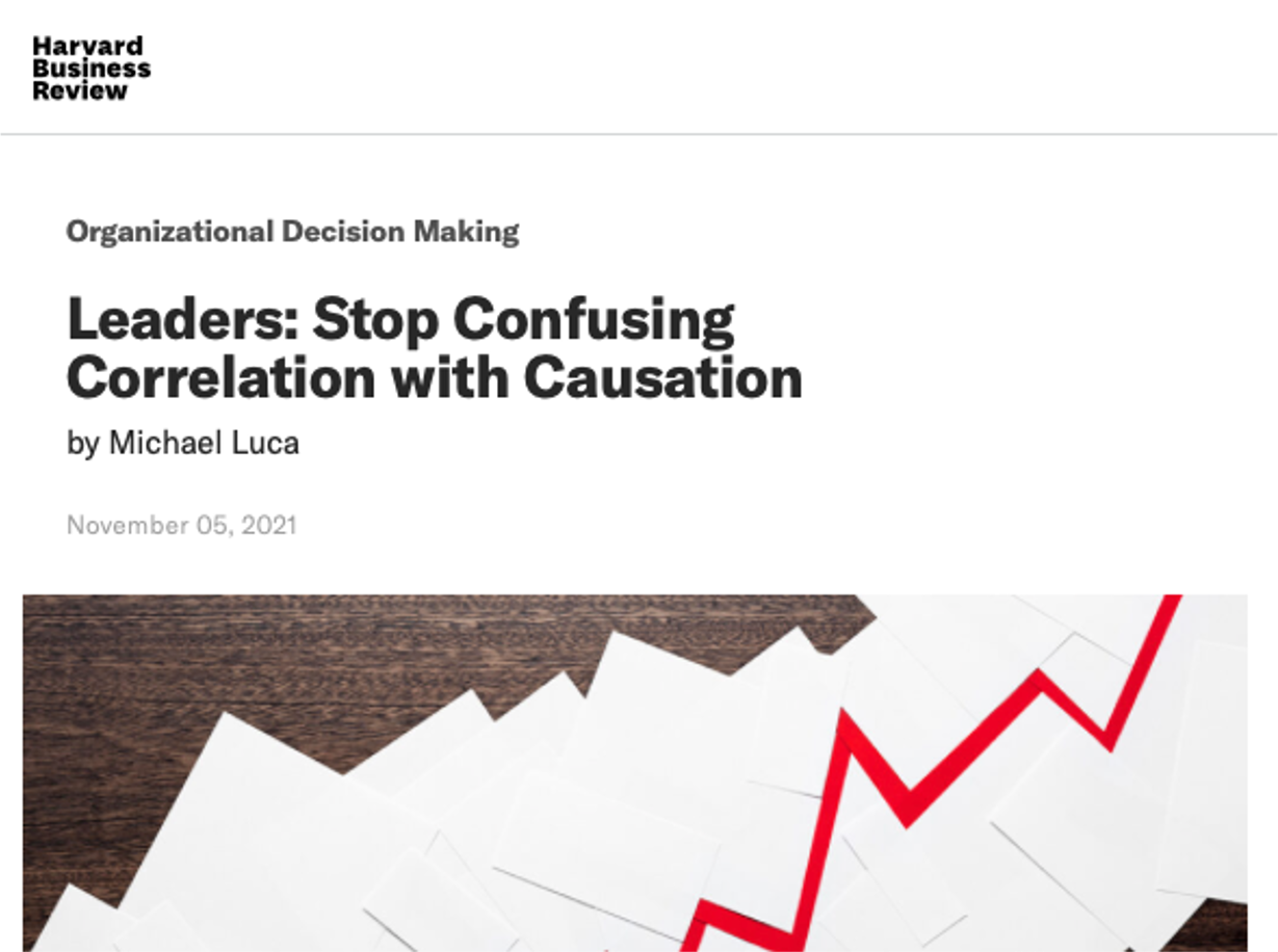
Leaders routinely confuse correlation with causation

Luca (2021)

Practitioner Evidence

Hünermund, Kaminski, and Schmitt (2022): Of 234 business practitioners surveyed, the vast majority use machine learning for decision problems that require causal, not correlational, answers — yet few apply causal methods.

This HBR article highlights a widespread problem in business analytics: leaders and data scientists routinely deploy predictive models for decision problems that are fundamentally causal in nature. The Hünermund et al. survey provides hard evidence — 234 practitioners were asked about their ML use cases, and the majority turned out to be causal questions dressed up as prediction tasks. This is not an academic concern; it leads to real misallocation of resources. We will see concrete examples throughout this session.

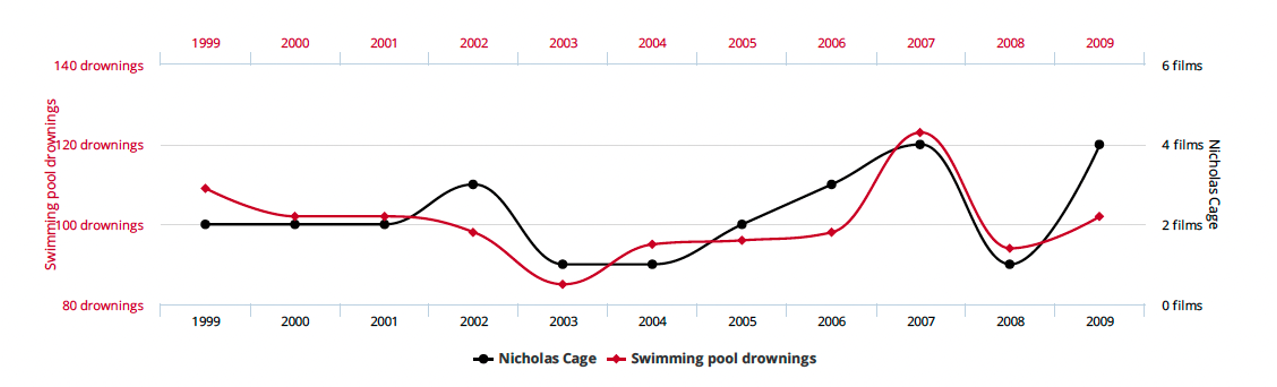
Spurious correlations look convincing until you see the mechanism

Nicolas Cage films vs. swimming pool drownings. Source: Tyler Vigen, Spurious Correlations

Tyler Vigen’s spurious correlations project is a memorable way to drive home the point. The correlation between Nicolas Cage films and swimming pool drownings is statistically real — the numbers check out. But no plausible mechanism connects these variables. This is a humorous example, but the same logic applies to serious business analytics: without a causal mechanism, even a strong correlation tells us nothing about what would happen if we intervened. Ask students: can you think of a business metric pair that correlates strongly but has no causal link?

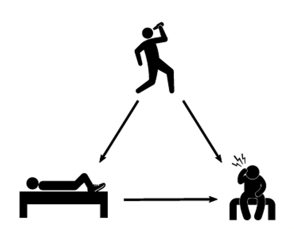
A common cause creates spurious association

The word for this is confounder: a common cause that creates a non-causal association between two variables.

Example: Drinking the night before is a common cause of both sleeping with shoes on and waking up with a headache. Shoes do not cause headaches.

Neal (2020)

We will formalize these diagrams in Session 02 using Directed Acyclic Graphs (DAGs). For now, treat arrows as direct causal effects. The headache example is intuitive: if you observe that people who sleep with shoes on tend to have headaches, you might naively conclude shoes cause headaches. But the real story is that a third variable — heavy drinking — causes both. This is confounding in its simplest form. Controlling for the confounder (drinking) eliminates the spurious association. The takeaway: whenever you see a correlation in business data, always ask “could there be a common cause?”

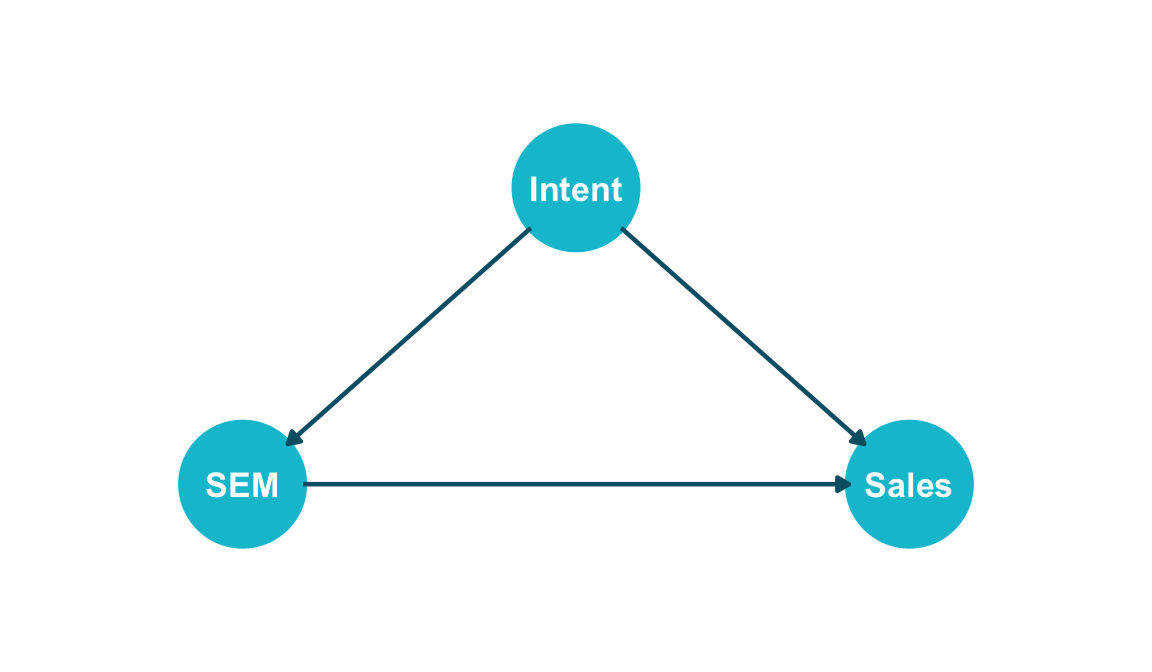
Even credible business data can mislead without causal reasoning

Blake, Nosko, and Tadelis (2015): eBay ran a large-scale experiment on branded search engine marketing (SEM) ads. They found that most of the “revenue” attributed to SEM was from consumers who would have purchased anyway. Consumers’ purchase intent is a common cause of both SEM ad clicks and sales.

library(ggdag)
library(ggplot2)

coord_dag <- list(
  x = c(SEM = 0, Intent = 0.5, Sales = 1),
  y = c(SEM = 0, Intent = 0.5, Sales = 0)
)

dag <- dagify(SEM ~ Intent,
              Sales ~ SEM,
              Sales ~ Intent,
              coords = coord_dag)

dag |>
  ggplot(aes(x = x, y = y, xend = xend, yend = yend)) +
  geom_dag_point(colour = "#00C1D4", size = 22) +
  geom_dag_edges(edge_colour = "#005e73", edge_width = 0.8) +
  geom_dag_text(colour = "white", size = 4.5, fontface = "bold") +
  expand_limits(x = c(-0.2, 1.2), y = c(-0.2, 0.7)) +
  coord_cartesian(clip = "off") +
  theme_dag(legend.position = "none")

Blake, Nosko, and Tadelis (2015)

The eBay example is one of the most famous case studies in causal inference for business. eBay was spending millions on branded search ads (ads that appear when users search for “eBay”). When they experimentally turned off ads in some markets, sales barely changed — because users who searched for “eBay” already intended to buy there. The observational data showed a strong correlation between ad spend and revenue, but the causal effect was near zero. This is confounding by purchase intent. The DAG shows the structure: Intent causes both SEM clicks and Sales. Without the experiment, eBay would never have discovered this. This motivates the entire course: we need formal tools to separate genuine causal effects from confounded associations.

Simpson’s Paradox

Google found it was underpaying… men?

“When Google conducted a pay study, it found it was underpaying men for similar work. The company […] increased compensation for thousands of male employees.” — The New York Times, March 2019

But wait — wasn’t Google just recently accused of discriminating against women?

“The US Department of Labor claims Google has systematically underpaid its female employees.” — The Verge, April 2017

How can the same company underpay both men and women? The answer lies in Simpson’s Paradox.

This is a real story that made headlines. The Department of Labor accused Google of systematically underpaying women. Two years later, Google’s own internal study concluded they were underpaying men. Both claims were based on data. How is this possible? This is Simpson’s Paradox in action — the direction of an association can reverse when you condition on (or ignore) a third variable. Let the class sit with the contradiction for a moment before moving to the numerical example.

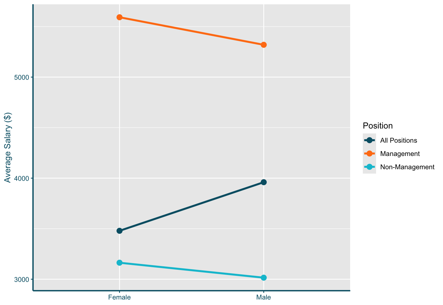
The same data, two opposite conclusions

Consider a simplified company with 100 women and 100 men:

	Women	Men
Non-Management	$3,163.30   (87 employees)	$3,015.18   (59 employees)
Management	$5,592.44   (13 employees)	$5,319.82   (41 employees)

Unadjusted gap (ignoring position):

\[\underbrace{\tfrac{87}{100} \times 3{,}163.30 + \tfrac{13}{100} \times 5{,}592.44}_{Women: \$3{,}479.09} \;-\; \underbrace{\tfrac{59}{100} \times 3{,}015.18 + \tfrac{41}{100} \times 5{,}319.82}_{Men: \$3{,}960.08} \;\approx\; -\$481\]

Adjusted gap — within each position, women earn more:

\[\underbrace{\tfrac{146}{200} \times (3{,}163.30 - 3{,}015.18)}_{\text{Non-Mgmt: } +\$108.13} \;+\; \underbrace{\tfrac{54}{200} \times (5{,}592.44 - 5{,}319.82)}_{\text{Mgmt: } +\$73.61} \;\approx\; +\$181.74\]

Which estimate gives us a more accurate picture?

Walk through the arithmetic step by step. The unadjusted comparison shows men earning ~$481 more on average. But when we look within each position level, women earn more in both categories. The reversal happens because men are disproportionately in higher-paying management roles (41% vs. 13%). So the aggregate comparison conflates the gender effect with the position effect. The adjusted figure of +$181.74 is a weighted average of the within-group differences. The critical question: which is the right number? The answer is — it depends on the causal structure. We need to know whether Position is a confounder or a mediator.

Subgroup and aggregate trends can point in opposite directions

library(ggplot2)

data <- data.frame(
  Salary = c(5319.82, 3015.18, 5592.44, 3163.30, 3960.08, 3479.09),
  Position = c("Management", "Non-Management", "Management",
               "Non-Management", "All Positions", "All Positions"),
  Gender = c("Male", "Male", "Female", "Female", "Male", "Female")
)

data |>
  ggplot(aes(x = Gender, y = Salary, group = Position, colour = Position)) +
  geom_line(linewidth = 1.2) +
  geom_point(size = 3) +
  labs(x = NULL, y = "Average Salary ($)", colour = "Position") +
  scale_colour_manual(values = c("All Positions" = "#005e73",
                                 "Management" = "#FF7E15",
                                 "Non-Management" = "#00C1D4")) +
  theme(axis.line = element_line(colour = "#005e73", linewidth = 0.8),
        axis.ticks = element_line(colour = "#005e73"),
        axis.text = element_text(colour = "#005e73"),
        axis.title = element_text(colour = "#005e73"))

The crossing pattern is the visual signature of Simpson’s Paradox: the aggregate trend reverses the subgroup trends.

The chart makes the paradox visually obvious. Within each position level, women earn more (the colored lines slope upward from Male to Female). But the aggregate line slopes downward because of the compositional imbalance — many more men are in the higher-paying Management group. Point out the crossing pattern: this is what Simpson’s Paradox looks like in a plot. The key insight is that neither the adjusted nor the unadjusted number is automatically correct. The right analysis depends on what we believe about the causal relationships between gender, position, and salary.

The answer depends on causal structure, not statistics

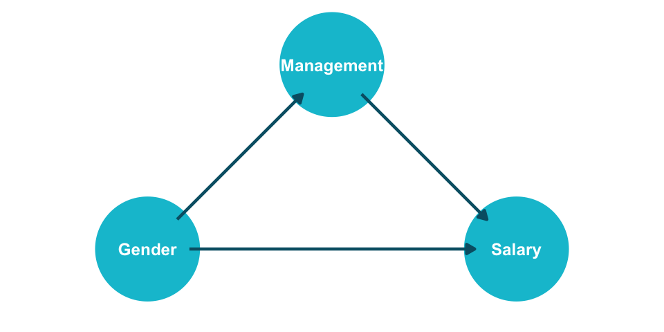
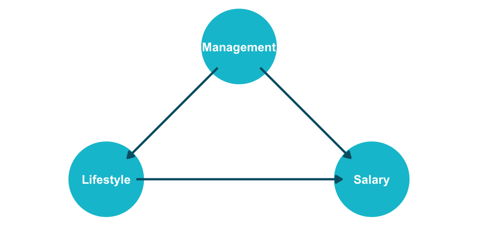
The same numbers could describe a completely different scenario. Replace “Gender” with “Lifestyle” and “Position” with “Management” — the joint distribution is identical.

Scenario 1: Gender → Position → Salary

Position is a mediator — do NOT adjust.

library(ggdag)
library(ggplot2)

coord_dag <- list(
  x = c(Gender = 0, Management = 0.5, Salary = 1),
  y = c(Gender = 0, Management = 0.5, Salary = 0)
)
dag <- dagify(Management ~ Gender,
              Salary ~ Gender,
              Salary ~ Management,
              coords = coord_dag)
dag |>
  ggplot(aes(x = x, y = y, xend = xend, yend = yend)) +
  geom_dag_point(colour = "#00C1D4", size = 26) +
  geom_dag_edges(edge_colour = "#005e73", edge_width = 0.8) +
  geom_dag_text(colour = "white", size = 3.2, fontface = "bold") +
  expand_limits(x = c(-0.25, 1.25), y = c(-0.15, 0.6)) +
  coord_cartesian(clip = "off") +
  theme_dag(legend.position = "none") +
  theme(plot.margin = margin(0, 0, 0, 0))

Scenario 2: Management → Lifestyle → Salary

Management is a confounder — DO adjust.

library(ggdag)
library(ggplot2)

coord_dag <- list(
  x = c(Lifestyle = 0, Management = 0.5, Salary = 1),
  y = c(Lifestyle = 0, Management = 0.5, Salary = 0)
)
dag <- dagify(Lifestyle ~ Management,
              Salary ~ Lifestyle,
              Salary ~ Management,
              coords = coord_dag)
dag |>
  ggplot(aes(x = x, y = y, xend = xend, yend = yend)) +
  geom_dag_point(colour = "#00C1D4", size = 26) +
  geom_dag_edges(edge_colour = "#005e73", edge_width = 0.8) +
  geom_dag_text(colour = "white", size = 3.2, fontface = "bold") +
  expand_limits(x = c(-0.25, 1.25), y = c(-0.15, 0.6)) +
  coord_cartesian(clip = "off") +
  theme_dag(legend.position = "none") +
  theme(plot.margin = margin(0, 0, 0, 0))

The joint distribution is identical. Statistics alone cannot tell you which analysis is correct.

This is the key slide of the Simpson’s Paradox section. Two structurally different causal stories produce the exact same data. In Scenario 1, gender causes position assignment (e.g., discriminatory promotion), so position is on the causal pathway — adjusting for it would block part of the effect we want to measure. In Scenario 2, management level is a common cause of both lifestyle and salary — it is a confounder that we should adjust for. The data cannot distinguish these scenarios. Only subject-matter knowledge about the causal mechanism can. This is why causal inference requires assumptions beyond the data. Emphasize: the numbers are identical, the correct analysis is opposite.

Statistics without causal assumptions is incomplete

1. Simpson’s Paradox: subgroup and aggregate trends can reverse — this is not a quirk but a structural feature of confounded data.

2. Whether to condition on a variable depends on its causal role (mediator vs. confounder) — not its statistical properties.

3. Causal assumptions are required for any analysis that goes beyond mere description. Statistics tells us what; causal inference tells us why and what if.

Transition: The potential outcomes framework gives us the formal language to state these assumptions precisely.

Summarize the three lessons from Simpson’s Paradox before moving to the formal framework. Point 1: the paradox is not rare or exotic — it arises whenever there is confounding and compositional imbalance. Point 2: the decision to adjust or not adjust is a causal decision, not a statistical one. Point 3: this means every data analysis implicitly makes causal assumptions, whether the analyst knows it or not. Better to make them explicit. The next section introduces the Rubin Causal Model (potential outcomes), which gives us the formal machinery to make these assumptions precise and derive their consequences.

Potential Outcomes

Causation requires a well-defined intervention

“No causation without manipulation.” — Rubin (1978); Holland (1986)

Treatments can be binary, multi-valued, or continuous:

• Take a drug vs. don’t take the drug
• Training program A vs. B vs. no training
• Amount of money spent on advertising (continuous)
• Race listed on a resume (Bertrand and Mullainathan 2004) — what counts as a “manipulation”?
• A person’s level of neuroticism? (Boundary case — hard to define an intervention)

The potential outcomes framework (Neyman 1990; Rubin 1974) formalizes causal questions by defining what would have happened under each possible treatment.

The manipulability criterion is central to the potential outcomes tradition. We can only ask a causal question if we can at least in principle imagine an intervention that changes the treatment. Drug trials are the clearest case. Advertising spend is continuous but still manipulable. The resume audit study (Bertrand & Mullainathan) pushes the boundary — race is not directly manipulable, but perceived race on a resume is. Neuroticism is even harder. This is where the framework has genuine limits. Holland (1986) coined the slogan “no causation without manipulation.” The Neyman-Rubin potential outcomes framework makes these ideas mathematically precise. We now define the notation.

Formal notation: units, treatments, and potential outcomes

• \(n\) units indexed by \(i = 1, \ldots, n\)
• \(Y\): outcome of interest
• \(D_i\): treatment assignment for unit \(i\) (binary: \(d_i \in \{0, 1\}\))

Potential outcomes:

• \(Y_i(1)\): the outcome unit \(i\) would experience if treated (\(D_i = 1\))
• \(Y_i(0)\): the outcome unit \(i\) would experience if not treated (\(D_i = 0\))

Individual Treatment Effect (ITE):

\[\tau_i = Y_i(1) - Y_i(0) \quad \forall \; i = 1, \ldots, n\]

Each unit has a pair of potential outcomes. The ITE compares them. The notation forces us to think about both possible states of the world.

Go through the notation carefully — students will use it for the rest of the course. The key conceptual shift: we think of each unit as having two potential outcomes simultaneously, one for each treatment condition. The ITE is the difference between these two. Note that tau_i is unit-specific — treatment effects can vary across individuals. This heterogeneity will become a major topic in Sessions 08-09. For now, just establish that the ITE is defined for every unit. The language of “would experience” is important: these are counterfactual quantities, not observed data.

SUTVA makes potential outcomes well-defined

For the potential outcomes \(Y_i(0)\) and \(Y_i(1)\) to be well-defined, we need:

Assumption 1: No Interference

Unit \(i\)’s potential outcomes do not depend on any other unit’s treatment assignment:

\[Y_i(d_1, d_2, \ldots, d_n) = Y_i(d_i)\]

Violated when: vaccination reduces disease for unvaccinated neighbors; a price change for one customer affects others’ behavior.

Assumption 2: Consistency (No Hidden Treatment Versions)

The observed outcome equals the potential outcome for the treatment actually received:

\[\text{If } D_i = d, \text{ then } Y_i = Y_i(d)\]

Violated when: “treatment” is ambiguous — e.g., “taking aspirin” could mean different doses, brands, or timing.

Assumption 3: SUTVA (Stable Unit Treatment Value Assumption)

Both Assumptions 1 and 2 hold: \(Y_i = Y_i(D_i)\). Under SUTVA, each unit has exactly two well-defined potential outcomes.

SUTVA is the foundation that makes the entire potential outcomes framework work. Walk through each component. No interference means unit i’s outcome depends only on its own treatment, not on what happens to other units. This is clearly violated in network settings (social media experiments, vaccination). Consistency means the treatment must be well-defined — “taking aspirin” needs to mean the same thing for everyone. Together they constitute SUTVA. When SUTVA holds, the potential outcomes are just two numbers per unit, clean and well-defined. When it is violated, we need more complex frameworks. For this course, we will mostly assume SUTVA holds unless stated otherwise. Ask: can you think of a business setting where no interference is clearly violated?

We never observe both potential outcomes for the same unit

Switching equation: \(\; Y_i = D_i \cdot Y_i(1) + (1 - D_i) \cdot Y_i(0)\)

We observe only the potential outcome corresponding to the treatment actually received.

\(i\)	\(D_i\)	\(Y_i\)	\(Y_i(1)\)	\(Y_i(0)\)	\(Y_i(1) - Y_i(0)\)
1	0	0	?	0	?
2	1	1	1	?	?
3	1	0	0	?	?
4	0	0	?	0	?
5	0	1	?	1	?
6	1	1	1	?	?

This is the Fundamental Problem of Causal Inference (Holland 1986): every individual treatment effect \(\tau_i\) requires a quantity we can never measure.

The switching equation makes the observability constraint concrete. When D=1, we see Y(1) and Y(0) is missing. When D=0, the reverse. The question marks in the table are not statistical uncertainty — they are logical impossibilities. Unit 1 was not treated, so we observe Y(0)=0, but we will never know what would have happened had they been treated. This is Holland’s Fundamental Problem. Individual causal effects are fundamentally unidentifiable from data alone. This seems devastating — but the next slides show how we can make progress by shifting from individual effects to average effects, under appropriate assumptions.

Can we salvage the situation by averaging?

Average Treatment Effect (ATE):

\[\tau = \mathbb{E}[\tau_i] = \mathbb{E}[Y_i(1) - Y_i(0)] = \mathbb{E}[Y_i(1)] - \mathbb{E}[Y_i(0)]\]

Or equivalently in finite-sample notation:

\[\tau = \frac{1}{n} \sum_{i=1}^{n} Y_i(1) \;-\; \frac{1}{n} \sum_{i=1}^{n} Y_i(0)\]

Still not computable — each sum requires all \(n\) values of \(Y(1)\) and all \(n\) values of \(Y(0)\), but we only observe one potential outcome per unit.

The counterfactuals are still missing. We need additional assumptions to make progress.

The natural move when individual effects are unidentifiable is to shift to population averages. The ATE asks: what is the average causal effect across all units? Linearity of expectation lets us decompose the expectation of the difference into a difference of expectations. But look at the sum form: to compute the first sum, we need Y_i(1) for every unit, including the untreated ones. Same problem. Averaging does not solve the fundamental problem — it just restates it at the population level. The key question becomes: under what assumptions can we replace the unobservable expectations E[Y(1)] and E[Y(0)] with computable quantities from our data? That is the identification problem, which we tackle next.

Under what assumptions can we identify causal effects from data?

Pause here. This is the central question of causal inference. Identification means: can we express a causal quantity (defined in terms of potential outcomes) as a function of observable data (joint distribution of treatments and outcomes)? If yes, we say the estimand is identified and we can then proceed to estimation. If no, no amount of data will help. The next section introduces the assumptions that make identification possible.

Identification

Ignorability: treatment assignment is as good as random

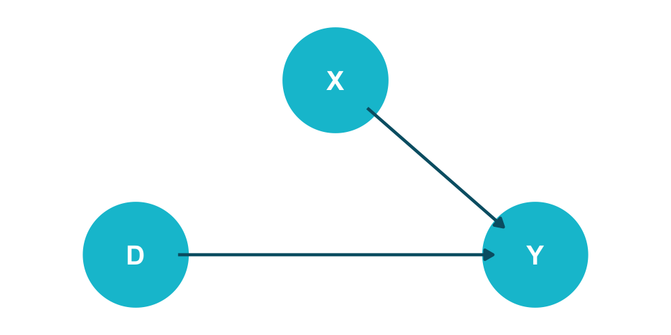
Assumption 4: Ignorability / Exchangeability / Unconfoundedness

\[(Y(1), Y(0)) \perp\!\!\!\perp D\]

The potential outcomes are statistically independent of treatment assignment. Intuitively: units in the treatment and control groups could be swapped without changing the outcome distributions.

library(ggdag)
library(ggplot2)

coord_dag <- list(
  x = c(D = 0, X = 0.5, Y = 1),
  y = c(D = 0, X = 0.5, Y = 0)
)
dag <- dagify(Y ~ D,
              Y ~ X,
              coords = coord_dag)
dag |>
  ggplot(aes(x = x, y = y, xend = xend, yend = yend)) +
  geom_dag_point(colour = "#00C1D4", size = 26) +
  geom_dag_edges(edge_colour = "#005e73", edge_width = 0.8) +
  geom_dag_text(colour = "white", size = 5, fontface = "bold") +
  expand_limits(x = c(-0.2, 1.2), y = c(-0.15, 0.65)) +
  coord_cartesian(clip = "off") +
  theme_dag(legend.position = "none") +
  theme(plot.margin = margin(0, 0, 0, 0))

Ignorability is the strongest and most important identification assumption. It says that treatment assignment carries no information about potential outcomes — as if treatment were assigned by coin flip. In an RCT, this holds by design. In observational data, it almost never holds unconditionally, because people select into treatment based on factors that also affect outcomes. The DAG shows the simplest case: D and Y are connected only through the causal arrow from D to Y, with no backdoor paths. If there were a confounder (a common cause of D and Y), ignorability would be violated. We will relax this to conditional ignorability on the next slides.

Under exchangeability, observed means identify causal effects

Using Assumptions 4 (exchangeability) and 2 (consistency):

\[\mathbb{E}[Y_i(1)] - \mathbb{E}[Y_i(0)] = \mathbb{E}[Y_i \mid D_i = 1] - \mathbb{E}[Y_i \mid D_i = 0]\]

The causal estimand (left) equals an associational estimand (right) that is computable from data.

\(i\)	\(D_i\)	\(Y_i\)	\(Y_i(1)\)	\(Y_i(0)\)
1	0	0	?	0
4	0	0	?	0
5	0	1	?	1
2	1	1	1	?
3	1	0	0	?
6	1	1	1	?

\(\hat{\mathbb{E}}[Y \mid D=1] = \frac{1+0+1}{3} = 0.67\), \(\quad \hat{\mathbb{E}}[Y \mid D=0] = \frac{0+0+1}{3} = 0.33\), \(\quad \widehat{ATE} = 0.33\)

Identification workflow: Causal Estimand → Statistical Estimand → Estimate.

This is the identification result. Under exchangeability, the group means of the treated and untreated units are valid estimates of the expectations of the potential outcomes. Walk through the table: we sort units by treatment status, compute the mean outcome in each group, and take the difference. The question marks are still there, but under exchangeability, the observed group means are unbiased for the population potential outcome means. The flowchart at the bottom summarizes the workflow: we start with a causal estimand (defined in potential outcomes), apply identification assumptions to obtain a statistical estimand (defined in observable data), then use estimation methods to get an estimate. This identification-estimation separation is fundamental to the course.

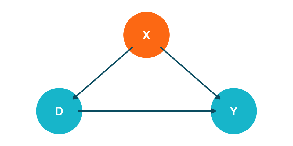
Conditional exchangeability makes ignorability realistic

Assumption 5: Conditional Ignorability / Conditional Exchangeability / Unconfoundedness

\[(Y(1), Y(0)) \perp\!\!\!\perp D \mid X\]

Potential outcomes are independent of treatment, conditional on observed covariates \(X\). Within strata defined by \(X\), treatment assignment is as good as random.

library(ggdag)
library(ggplot2)

coord_dag <- list(
  x = c(D = 0, X = 0.5, Y = 1),
  y = c(D = 0, X = 0.5, Y = 0)
)
dag <- dagify(Y ~ D,
              Y ~ X,
              D ~ X,
              coords = coord_dag)

dag_data <- dag |> tidy_dagitty()
dag_data$data$colour <- ifelse(dag_data$data$name == "X", "#FF7E15", "#00C1D4")

dag_data |>
  ggplot(aes(x = x, y = y, xend = xend, yend = yend)) +
  geom_dag_point(aes(colour = colour), size = 26) +
  scale_colour_identity() +
  geom_dag_edges(edge_colour = "#005e73", edge_width = 0.8) +
  geom_dag_text(colour = "white", size = 5, fontface = "bold") +
  expand_limits(x = c(-0.2, 1.2), y = c(-0.15, 0.65)) +
  coord_cartesian(clip = "off") +
  theme_dag(legend.position = "none") +
  theme(plot.margin = margin(0, 0, 0, 0))

Conditional exchangeability is the practical version of ignorability: we allow confounders, but assume we have measured all of them in X. Within each stratum of X, treatment assignment behaves as if random. The DAG shows X as a common cause of D and Y. X is highlighted in orange to indicate that we condition on it, which blocks the backdoor path.

Positivity ensures we can estimate both counterfactuals

Assumption 6: Positivity / Overlap / Common Support

\[0 < P(D = 1 \mid X = x) < 1 \quad \text{for all } x \text{ with } P(X = x) > 0\]

Every subgroup defined by \(X\) must contain both treated and untreated units.

Trade-off: conditioning on more covariates helps unconfoundedness but can hurt positivity — adding variables to \(X\) increases the risk of empty strata.

Positivity is the complementary requirement: even after conditioning on X, there must be both treated and untreated units in every stratum. Without positivity, we cannot estimate the counterfactual for one of the groups. There is an inherent tension: adding more variables to X makes unconfoundedness more plausible but increases the risk of empty strata (positivity violations). This trade-off is central to methods like matching, propensity scores, and double ML covered in later sessions.

The ATE is identified under four assumptions

Theorem: Identification of the ATE

Under conditional unconfoundedness, positivity, consistency, and no interference:

\[\tau = \mathbb{E}_X\!\Big[\mathbb{E}[Y_i \mid D_i = 1, X_i] - \mathbb{E}[Y_i \mid D_i = 0, X_i]\Big]\]

The outer expectation \(\mathbb{E}_X\) averages the conditional treatment effects over the distribution of \(X\) in the population. This is the adjustment formula — the foundation for regression, matching, IPW, and double ML.

Required assumptions:

1. Conditional unconfoundedness (Assumption 5): \((Y(1), Y(0)) \perp\!\!\!\perp D \mid X\)
2. Positivity (Assumption 6): \(0 < P(D=1 \mid X=x) < 1\) for all relevant \(x\)
3. Consistency (Assumption 2): \(D_i = d \Rightarrow Y_i = Y_i(d)\)
4. No interference (Assumption 1): \(Y_i(d_1, \ldots, d_n) = Y_i(d_i)\)

This is the central identification theorem of the course. State it clearly and connect back to the assumptions we have built up. The formula says: compute the conditional mean difference within each stratum of X, then average over the distribution of X. The outer expectation ensures we weight subgroups by their prevalence in the population. This formula is the foundation for virtually every causal estimation method in the course. Regression adjustment estimates it parametrically. Matching does it nonparametrically by finding similar units. Inverse probability weighting reweights the sample to mimic exchangeability. Double ML uses flexible ML models for the conditional expectations. All of these are different estimators for the same identified estimand. The proof on the next slide shows exactly how the four assumptions combine.

From potential outcomes to observable data in four steps

\[ \begin{align*} \tau = \mathbb{E}[\tau_i] &= \mathbb{E}[Y_i(1) - Y_i(0)] \\ &= \mathbb{E}[Y_i(1)] - \mathbb{E}[Y_i(0)] \\ & \color{#00C1D4}{\text{(linearity of expectation)}} \\ &= \mathbb{E}_X [\mathbb{E}[Y_i(1) \mid X_i]] - \mathbb{E}_X [\mathbb{E}[Y_i(0) \mid X_i]] \\ &\color{#00C1D4}{\text{(law of iterated expectations)}} \\ &= \mathbb{E}_X [\mathbb{E}[Y_i(1) \mid D_i = 1, X_i]] - \mathbb{E}_X [\mathbb{E}[Y_i(0) \mid D_i = 0, X_i]] \\ &\color{#00C1D4}{\text{(unconfoundedness and positivity)}} \\ &= \mathbb{E}_X [\mathbb{E}[Y_i \mid D_i = 1, X_i]] - \mathbb{E}_X [\mathbb{E}[Y_i \mid D_i = 0, X_i]] \\ &\color{#00C1D4}{\text{(consistency)}} \end{align*} \]

Each step uses exactly one assumption. The final line contains only observable quantities.

Walk through each step of the proof. Line 1 to 2: linearity of expectation decomposes the difference of potential outcomes. Line 2 to 3: the law of iterated expectations introduces conditioning on X — this is where the outer expectation comes from. Line 3 to 4: conditional unconfoundedness allows us to add the conditioning on D — because potential outcomes are independent of D given X, knowing D does not change the conditional expectation. Positivity ensures these conditional expectations exist (no empty cells). Line 4 to 5: consistency replaces Y(d) with the observed Y for units where D=d. The final expression is entirely in terms of observable quantities: we can estimate each conditional mean from data. This proof is the conceptual backbone of the course. Encourage students to revisit it when they encounter specific estimation methods later.

Now we know what to estimate — but which quantity matters for your decision?

Brief transition to the final section. We have established that the ATE is identifiable. But in practice, different stakeholders care about different estimands. A policymaker might want the ATE (population-wide effect). A firm might want the ATT (effect for those who actually adopted the treatment). A doctor might want the CATE (effect for a specific patient subgroup). The last section introduces these variants and previews how they connect to the rest of the course.

Estimands

The ATT asks what treatment did for those who received it

Average Treatment Effect on the Treated (ATT)

\[ATT = \mathbb{E}[Y_i(1) \mid D_i = 1] - \mathbb{E}[Y_i(0) \mid D_i = 1]\]

Business example: A company ran a loyalty program. The ATT answers: how much did the program benefit enrolled customers? The counterfactual is what they would have spent without the program.

Average Treatment Effect on the Control (ATC)

\[ATC = \mathbb{E}[Y_i(1) \mid D_i = 0] - \mathbb{E}[Y_i(0) \mid D_i = 0]\]

Decomposition: The ATE is a weighted average of ATT and ATC:

\[ATE = P(D=1) \cdot ATT + P(D=0) \cdot ATC\]

When \(ATT \neq ATC\), we have treatment effect heterogeneity by treatment status — those who select into treatment may benefit differently.

The ATT is often the most policy-relevant estimand. When a company evaluates a program, they care about the effect on participants, not on the entire population. The loyalty program example: we observe that enrolled customers spent more, but would they have spent more anyway (selection bias)? The ATT isolates the program effect for this specific group. The ATC asks the complementary question: what would happen if non-participants were forced into the program? The decomposition shows that ATE = weighted average of ATT and ATC. If ATT = ATC, there is no treatment effect heterogeneity by selection status. If they differ, it matters which estimand you report. In many business contexts, ATT and ATE differ substantially because of self-selection.

Treatment effects vary — CATE reveals who benefits most

Conditional Average Treatment Effect (CATE)

\[CATE(x) = \mathbb{E}[Y_i(1) \mid X_i = x] - \mathbb{E}[Y_i(0) \mid X_i = x]\]

The treatment effect for the subpopulation with covariates \(X = x\).

Business example: A new drug has a positive ATE on average. But which patients benefit most? CATE estimation reveals treatment effect heterogeneity across patient characteristics.

Industry application: Feuerriegel, Shrestha, and Krogh (2025) report that ABB Hitachi used CATE-based targeting to allocate quality interventions in manufacturing — cutting yield loss by half compared to a uniform treatment rule.

Course preview: Treatment effect heterogeneity is the focus of Sessions 08–09, where we cover Double Machine Learning and Causal Forests for flexible CATE estimation.

The CATE is where causal inference meets personalization. Instead of asking “does the treatment work on average,” we ask “for whom does it work best?” This is critical for targeting in marketing, precision medicine, and manufacturing. The Feuerriegel et al. case study is compelling: ABB Hitachi could not afford to apply quality interventions to every unit on the production line, so they used CATE estimates to target interventions where they would have the largest impact on yield. The result was a 50% reduction in yield loss. This is the promise of heterogeneous treatment effect estimation. We will cover the methods — Double Machine Learning, Causal Forests, meta-learners — in the second half of the course. For now, just plant the seed that treatment effects are not one number but a function of covariates.

Key Takeaways

1. Causal questions require causal assumptions — statistics alone is not enough. Simpson’s Paradox shows that the same data supports opposite conclusions depending on causal structure.

2. The potential outcomes framework formalizes causality as a missing data problem. Each unit has two potential outcomes; we observe only one. Individual treatment effects are fundamentally unidentifiable.

3. Under ignorability + positivity + consistency, causal effects become identifiable from observational data. The adjustment formula translates causal estimands into statistical estimands that we can estimate.

Next session: We formalize causal assumptions using Directed Acyclic Graphs (DAGs) — a visual language for encoding what we believe about the data-generating process.

Wrap up by connecting the three main threads of the lecture. Thread 1 (Motivation + Simpson’s Paradox): correlation is not causation, and the decision of what to adjust for requires causal knowledge. Thread 2 (Potential Outcomes): the formal framework that defines treatment effects as comparisons of counterfactual states. Thread 3 (Identification): the assumptions under which we can bridge the gap from causal estimands to statistical estimands. Preview Session 02: DAGs give us a graphical language to encode and reason about causal assumptions. They will tell us which variables to adjust for and which to leave alone — resolving Simpson’s Paradox systematically. Encourage students to read Chapter 1 of Neal (2020) or Cunningham (2021) before next session.

References

Bertrand, Marianne, and Sendhil Mullainathan. 2004. “Are Emily and Greg More Employable Than Lakisha and Jamal? A Field Experiment on Labor Market Discrimination.” American Economic Review 94 (4): 991–1013. https://doi.org/10.1257/0002828042002561.

Blake, Thomas, Chris Nosko, and Steven Tadelis. 2015. “Consumer Heterogeneity and Paid Search Effectiveness: A Large-Scale Field Experiment.” Econometrica 83 (1): 155–74. https://doi.org/10.3982/ECTA12423.

Feuerriegel, Stefan, Yash Raj Shrestha, and Georg von Krogh. 2025. “A New Machine Learning Approach Answers What-If Questions.” MIT Sloan Management Review 66 (3): 65–69. https://sloanreview.mit.edu/article/a-new-machine-learning-approach-answers-what-if-questions/.

Holland, Paul W. 1986. “Statistics and Causal Inference.” Journal of the American Statistical Association 81 (396): 945–60. https://doi.org/10.1080/01621459.1986.10478354.

Hünermund, Paul, Jermain Kaminski, and Carla Schmitt. 2022. “Causal Machine Learning and Business Decision Making.” SSRN Working Paper. https://doi.org/10.2139/ssrn.3867326.

Luca, Michael. 2021. “Leaders: Stop Confusing Correlation with Causation.” Harvard Business Review. https://hbr.org/2021/11/leaders-stop-confusing-correlation-with-causation.

Neal, Brady. 2020. Introduction to Causal Inference from a Machine Learning Perspective. Course Lecture Notes (draft). https://www.bradyneal.com/causal-inference-course.

Neyman, Jerzy. 1990. “On the Application of Probability Theory to Agricultural Experiments. Essay on Principles. Section 9.” Statistical Science 5 (4): 465–72. https://doi.org/10.1214/ss/1177012031.

Rubin, Donald B. 1974. “Estimating Causal Effects of Treatments in Randomized and Nonrandomized Studies.” Journal of Educational Psychology 66 (5): 688–701. https://doi.org/10.1037/h0037350.

———. 1978. “Bayesian Inference for Causal Effects: The Role of Randomization.” The Annals of Statistics 6 (1): 34–58. https://www.jstor.org/stable/2958688.

Thank you for your attention!
	www.startupengineer.io/team/ihl/ christoph-ihl christophihl